Project-1: Modelling an electric Car with Li-ion battery
Aim:
Create a MATLAB model of electric car which uses lithium ion battery and suitable motor. Choose suitable blocks from Simscape or Powertrain block set. Implement the vehicle speed control using PI controller and generate brake and accelerator commands. Avoid using readymade driver block for speed control.
Objectives:
Design the Vehicle speed control using the PI controller and generate Brake and acceleration commands.
Run the model with theDrive cycle and observe the Distance travelled, Soc and velocity of the vechicle.
System Level Configuration:
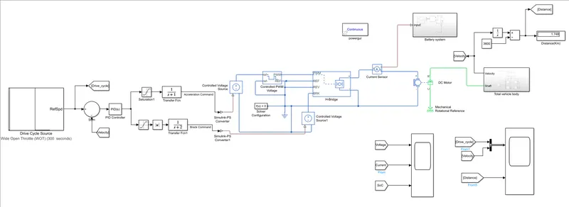
The entire model is divided in to 4 parts
- Toatl Vehicle Body
- Motor and controller
- Battery
- Driver and drive cycle
1.Total Vehicle Body:
It is created as a subsystem
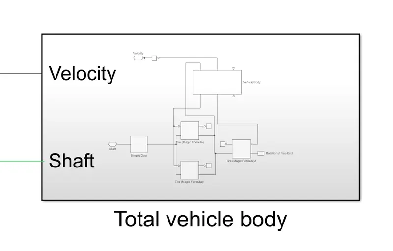
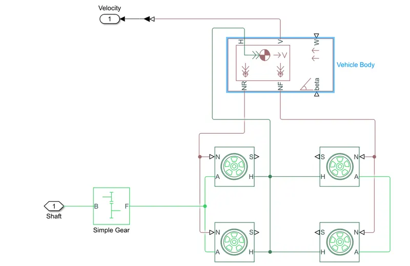
It is Rear wheel Drive. The motor axil is connected to the Rare wheels axil.
It is a combination of different parts
- vehicle body
- Wheels
- Simple gear
Vehicle body:
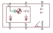
The Vehicle Body block represents a two-axle vehicle body in longitudinal motion. The vehicle can have the same or a different number of wheels on each axle. For example, two wheels on the front axle and one wheel on the rear axle. The vehicle wheels are assumed identical in size. The vehicle can also have a center of gravity (CG) that is at or below the plane of travel.
The block accounts for body mass, aerodynamic drag, road incline, and weight distribution between axles due to acceleration and road profile. Optionally include pitch and suspension dynamics. The vehicle does not move vertically relative to the ground.
The block has an option to include an externally-defined mass and an externally-defined inertia. The mass, inertia, and center of gravity of the vehicle body can vary over the course of simulation in response to system changes.
Inputs:
W = head wind speed = 0 m/s (let us assume it has no opp wind speed)
Beta = Road incline angle = 0 rad (let us assume there is no road inclination)
H = Horizontal motion - Connect tire traction motion to this port.
Output:
NR = Rear axil normal force (N)
FR = front axil normal force (N)
V = Velocity (m/s)
Input parameters:
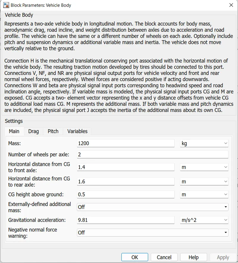 \
\
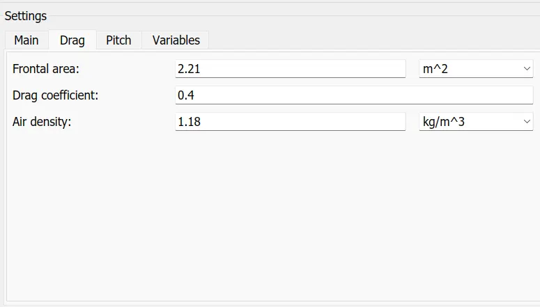
All other are default values
wheels:

The Tire (Magic Formula) block models a tire with longitudinal behavior given by the Magic Formula [1], an empirical equation based on four fitting coefficients. The block can model tire dynamics under constant or variable pavement conditions.
The longitudinal direction of the tire is the same as its direction of motion as it rolls on pavement. This block is a structural component based on the Tire-road Interaction (Magic Formula) block.
To increase the fidelity of the tire model, you can specify properties such as tire compliance, inertia, and rolling resistance. However, these properties increase the complexity of the tire model and can slow down simulation. Consider ignoring tire compliance and inertia if simulating the model in real time or if preparing the model for hardware-in-the-loop (HIL) simulation.
A = Axil
H = Hub
S = slip = 0
N = Normal force
input parameters:
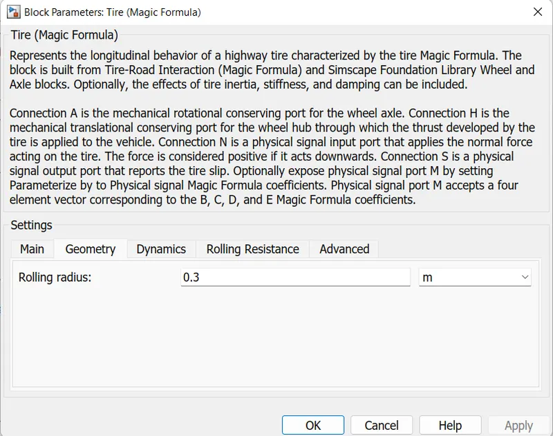
All other parameters are default values
Simple gear:

The Simple Gear block represents a gearbox that constrains the connected driveline axes of the base gear, B, and the follower gear, F, to corotate with a fixed ratio that you specify. You choose whether the follower axis rotates in the same or opposite direction as the base axis. If they rotate in the same direction, the angular velocity of the follower, ωF, and the angular velocity of the base, ωB, have the same sign. If they rotate in opposite directions, ωF and ωB have opposite signs.
F = Follower = Rotational mechanical conserving port associated with the follower, or output, shaft.
B = base = Rotational mechanical conserving port associated with the base, or input, shaft. It is connected to the motor Output
Input parameters:
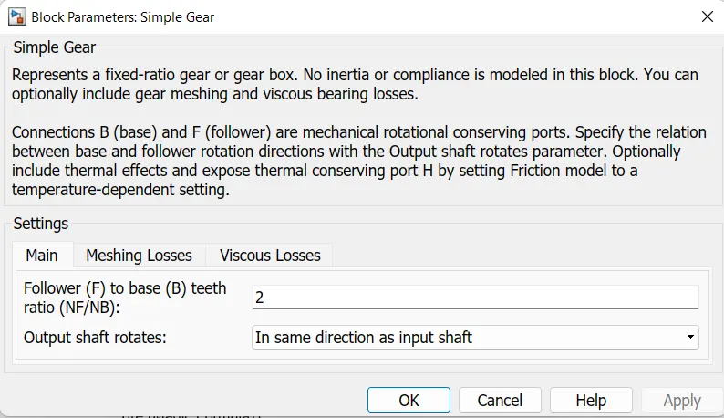
Other blocks are
Terminator

Use the PS Terminator block to cap physical signal output ports that do not connect to other blocks.
Unlike conserving ports in physical modeling, or Simulink® output ports, unconnected physical signal output ports do not generate warnings. However, you can use a PS Terminator block for clarity, to indicate that the signal was not inadvertently left unconnected.
As the slip is considered as zero it should be terminated using the terminator
2. Motor and controller:
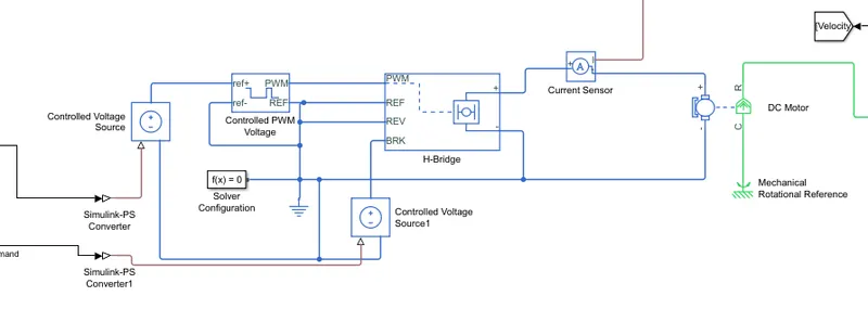
It is combination of
- DC motor
- H-Bridge
- Controlled PWM Voltage
- Controlled volatge source
- Current sensor
DC Motor:
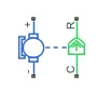
R = motor rotor = it is connected to shaft of the vehicle body
C = case = Mechanical rotational conserving port associated with the DC motor case, as it is stationary part it is conneted to Mechanical Rotational Referance
+ = positive termial of the motor, connected to H-Bridge output + termial
- = Negitive termial of the motor, connected to H-Bridge output - termial
The parameters are taken as
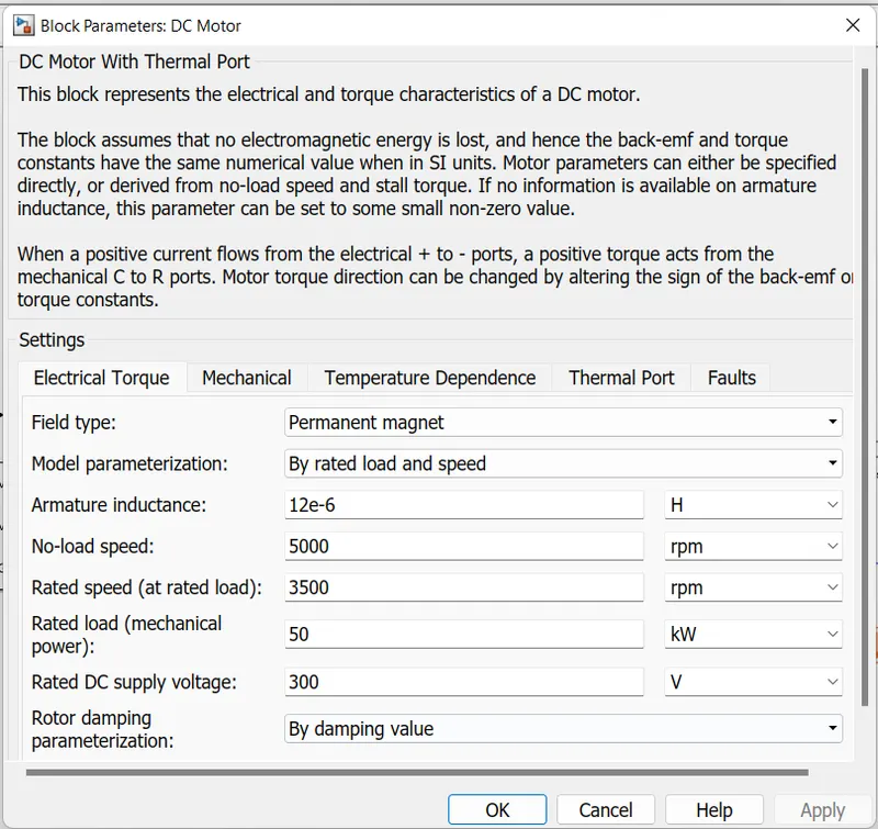
All other parameters are taken default values.
H-Bridge:
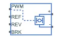
It is used to control the Motor speed and direction accorting to the drive cycle.
+ = Positive terminal of the H-Bridge, It is a output of the H-bridge connected to + of the motor
- = Negitive terminal of the H-Bridge, It is a output of the H-bridge connected to - of the motor
PWM = input signal, it is connected to the PWM pulse generater
REF = Referance, it is connected to Electrical ground
REV = Reverse of the motor, it is connected to ground because we are assuming that vehicle is going only in one froward direction.
BRK = Break, it is connected to the Driver through the Controlled voltage source.
Its parameters are taken as:
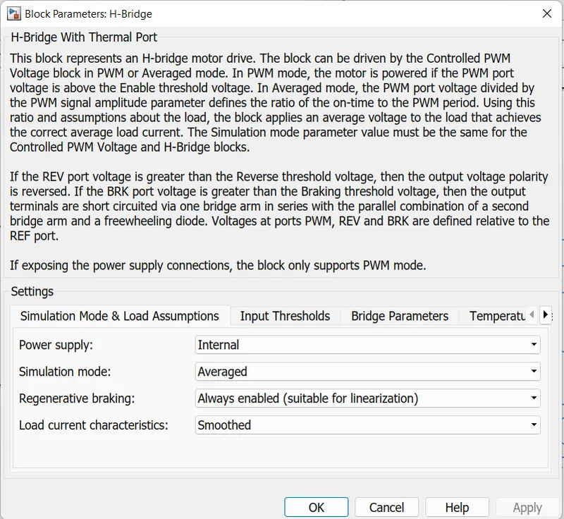
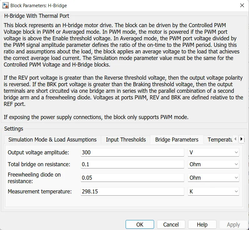
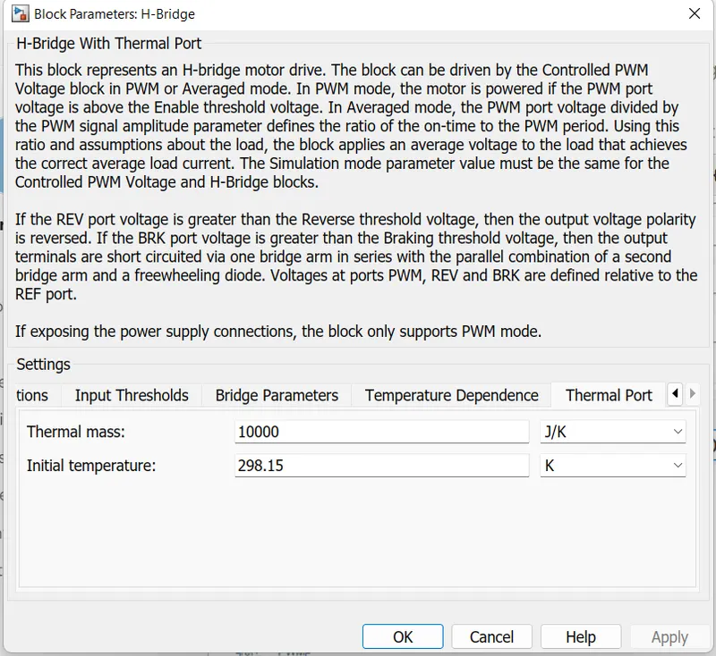
All other parameters are taken as defult values.
Controlled PWM Voltage:

PWM = Pulse output, connected to H-Bridge PWM port. It geneartes the requried duty cycle for the H-Bridge according to the Drive Cycle.
REF = referance , it is connected to the electrical referance
ref+ = Referance voltage, it is the drive cycle referance voltage input
ref- = ground
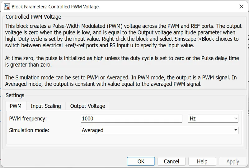
All other parameters are taken as default values.
Controlled Voltage Source:

The Controlled Voltage Source block represents an ideal voltage source that is powerful enough to maintain the specified voltage at its output regardless of the current flowing through the source.
The output voltage is V = Vs, where Vs is the numerical value presented at the physical signal port.
Generates the voltage from driver for the Controlled PWM Voltage referance voltage, so that the Controlled PWM Voltage can generate the Duty cycle as required
Signal port is connected to the Longitudinal Driver Aceleration port. Another Controlled voltage source signal port is connected to Longitudinal Driver deceleration port. So that the required voltage is generated for Acceleration and deceleration for H- Bridge.
Current Sensor:

The Current Sensor block represents an ideal current sensor, that is, a device that converts current measured in any electrical branch into a physical signal proportional to the current.
Connections + and – are electrical conserving ports through which the sensor is inserted into the circuit. Connection I is a physical signal port that outputs the measurement result.
Used to measure the current flowing through the Motor.
Electrical referance:

The Electrical Reference block represents an electrical ground. Electrical conserving ports of all the blocks that are directly connected to ground must be connected to an Electrical Reference block. A model with electrical elements must contain at least one Electrical Reference block.
Solver Configuration:

Each physical network represented by a connected Simscape™ block diagram requires solver settings information for simulation. The Solver Configuration block specifies the solver parameters that your model needs before you can begin simulation.
Each topologically distinct Simscape block diagram requires exactly one Solver Configuration block to be connected to it.
3. Battery:
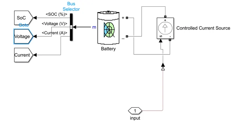
3. Battery:
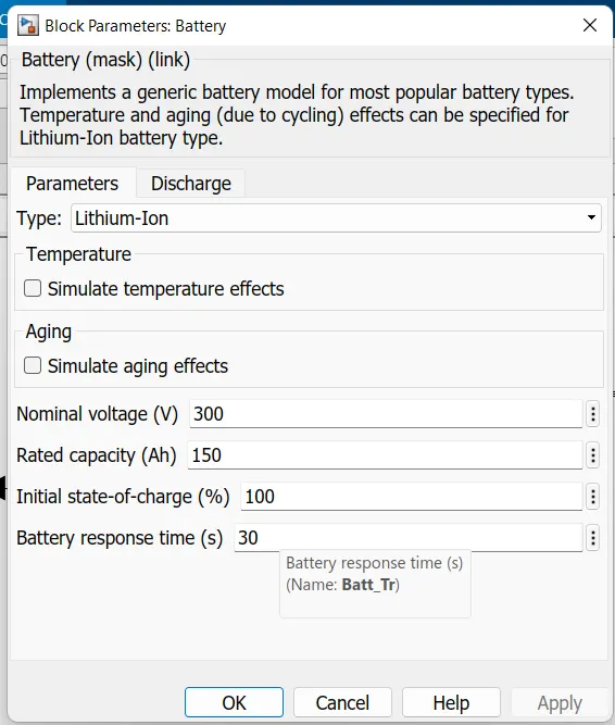
The Battery block implements a generic dynamic model that represents most popular types of rechargeable batteries.
The blockparameters:
Energy calculation is done by the formula P⋅t1000">P⋅t1000P⋅t1000 KWh
Power (P) = Voltage * Current
integrating it gives the Energy consmption in Watts and dividing it with 3600 gives Watt-Hour
Controlled Current Source:

The Controlled Current Source block converts the Simulink® input signal into an equivalent current source. The generated current is driven by the input signal of the block. The positive current direction is as shown by the arrow in the block icon.
You can initialize the Controlled Current Source block with a specific AC or DC current. If you want to start the simulation in steady state, the block input must be connected to a signal starting as a sinusoidal or DC waveform corresponding to the initial values.
It gets the control single from the H-Bridge current measurnment block.
4. Driver and drive cycle:
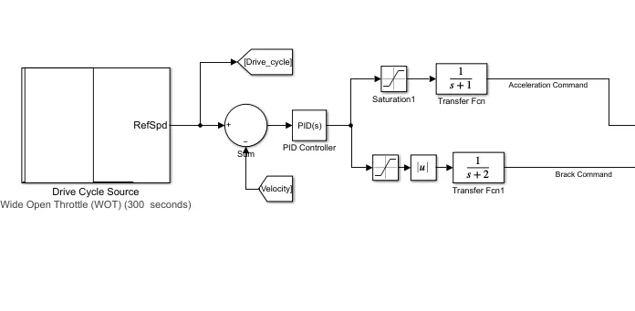
Driver:
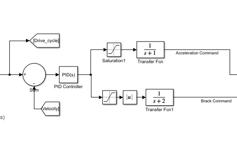
It is designed from Sum,PID,Stauratan and Transfer function block.
Sum:

The Sum block performs addition or subtraction on its inputs. The Add, Subtract, Sum of Elements, and Sum blocks are identical blocks. This block can add or subtract scalar, vector, or matrix inputs. It can also collapse the elements of a signal and perform a summation.
You specify the operations of the block with the List of signs parameter with plus (+), minus (-), and spacer (|).
-
The number of
+and-characters equals the number of inputs. For example,+-+requires three inputs. The block subtracts the second (middle) input from the first (top) input, and then adds the third (bottom) input. -
A spacer character creates extra space between ports on the block icon.
-
If performing only addition, you can use a numerical value equal to the number of inputs.
-
If only there is only one input port, a single
+or-adds or subtracts the elements over all dimensions or in the specified dimension.
The Sum block first converts the input data type to its accumulator data type, then performs the specified operations. The block converts the result to its output data type using the specified rounding and overflow modes.
In this model the signs are taken as +- . The + for drive cycle which is referance speed and negitive for vehicle speed which is feedback. the sum block gives the error speed to PID controller.
PID:
The Discrete PID Controller block implements a PID controller (PID, PI, PD, P only, or I only). The block is identical to the PID Controller block with the Time domain parameter set to Discrete-time.
The block output is a weighted sum of the input signal, the integral of the input signal, and the derivative of the input signal. The weights are the proportional, integral, and derivative gain parameters. A first-order pole filters the derivative action.
The block supports several controller types and structures. Configurable options in the block include:
-
Controller type (PID, PI, PD, P only, or I only) — See the Controller parameter.
-
Controller form (Parallel or Ideal) — See the Form parameter.
-
Time domain (continuous or discrete) — See the Time domain parameter.
-
Initial conditions and reset trigger — See the Source and External reset parameters.
-
Output saturation limits and built-in anti-windup mechanism — See the Limit output parameter.
-
Signal tracking for bumpless control transfer and multiloop control — See the Enable tracking mode parameter.
As you change these options, the internal structure of the block changes by activating different variant subsystems. (For more information, see Variant Subsystems). To examine the internal structure of the block and its variant subsystems, right-click the block and select Mask > Look Under Mask.
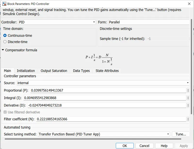
Here the P,I and D values are founf from the Autotuning the PID control by using the Transfer function base tuning and the values are found to be as shown below
Saturation:

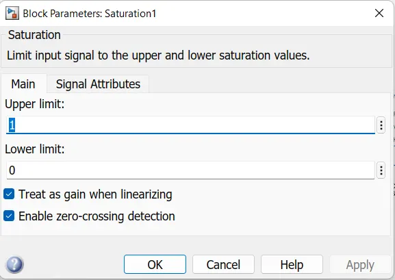
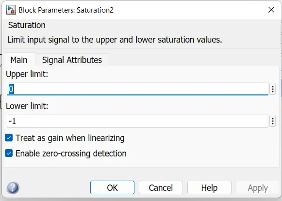
The Saturation block produces an output signal that is the value of the input signal bounded to the upper and lower saturation values. The upper and lower limits are specified by the parameters Upper limit and Lower limit.
Here we used the 2 saturaion blockes one for Acceleration and other for Braking as shown above. This will sparate the Acceleration signal and deceleration signal and give it to the Transfer function.
Acceleration:
Braking:
Abs block:

The Abs block outputs the absolute value of the input.
It will convert the negitive Brack signal to positive signal, and give it to the transfer function.
Transfer fun:

The Transfer Fcn block models a linear system by a transfer function of the Laplace-domain variable s. The block can model single-input single-output (SISO) and single-input multiple-output (SIMO) systems.
It will creat the base Transfer function foe the Acceleration and Brack. We use the 2 tarnsfer fun blocks one for Acceleration and another for Brake.
For Acceleration the transfer function is given by
`1/(s+1)`
This output give the Acceleration Command
For Brake the transfer function is given by
`1/(s+2)`
This output give the Brake Command
Drive cycles:
The Drive Cycle Source block generates a standard or user-specified longitudinal drive cycle. The block output is the specified vehicle longitudinal speed, which you can use to:
-
Predict the engine torque and fuel consumption that a vehicle requires to achieve desired speed and acceleration for a given gear shift reference.
-
Produce realistic velocity and shift references for closed loop acceleration and braking commands for vehicle control and plant models.
-
Study, tune, and optimize vehicle control, system performance, and system robustness over multiple drive cycles.
-
Identify the faults within tolerances specified by standardized tests, including:
-
EPA dynamometer driving schedules1
-
Worldwide Harmonised Light Vehicle Test Procedure (WLTP) laboratory tests2
-
For the drive cycles, you can use:
-
Drive cycles from predefined sources. By default, the block includes the
FTP–75drive cycle. To install additional drive cycles from a support package, see Instal Drive Cycle. The support package has drive cycles that include the gear shift schedules, for exampleJC08andCUEDC. -
Workspace variables that define your own drive cycles.
-
.
mat, .xls, .xlsx, or .txtfiles. -
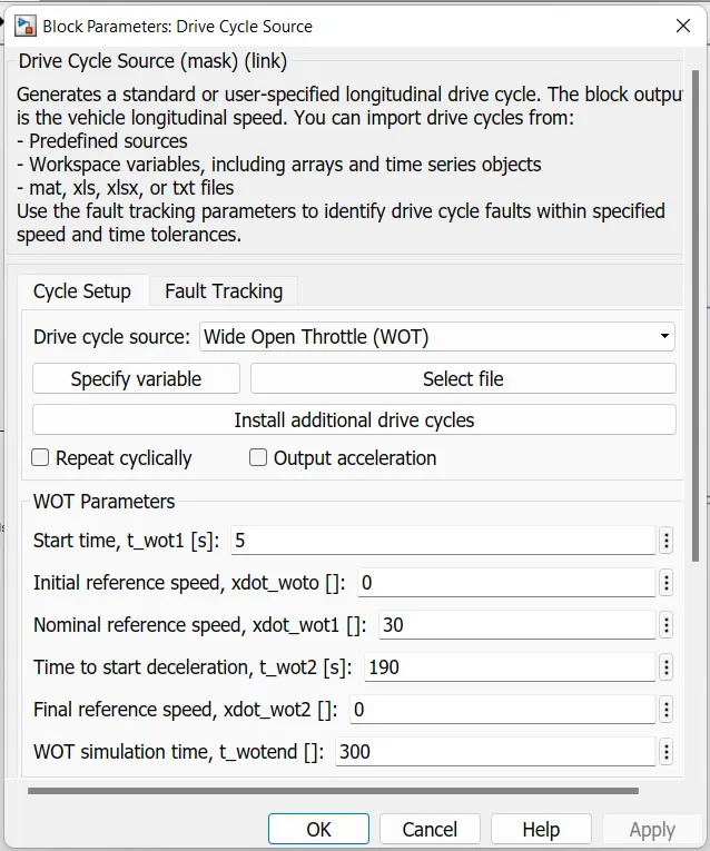
Wide open throttle (WOT) parameters, including initial and nominal reference speed, deceleration start time, and final reference speed.
WOT Drive Cycle:
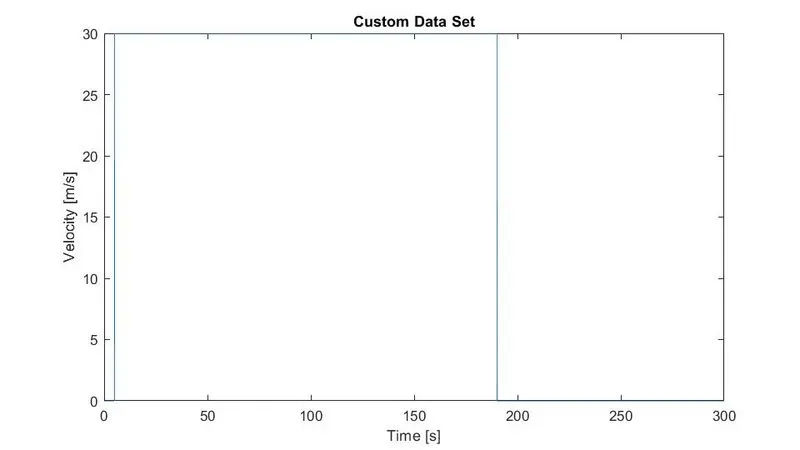
The prarameters are given by
Results:
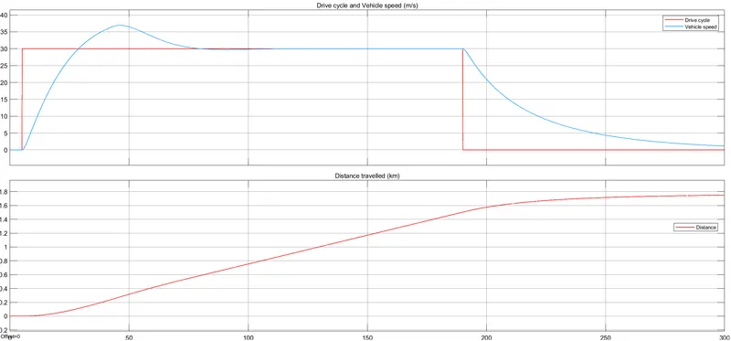
The vechicle is following the WOT cycle and it is stabled at around 70 sec. If we use other methods like adding inintigrator,lead compensator or lag compensator it will come to stable state with in short time.
The Distance travelled by the vehicle with 30m/s for 190 sec acceleration is 1.748 Km.
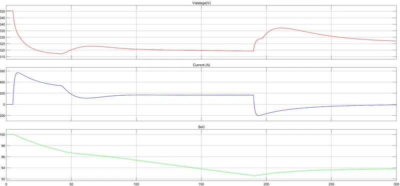
The Volatge of the battery is changing with the drive cycle and it is controlled by the Acceleration and Brake command
The current of the battery is changing with the drive cycle and it is controlled by the Acceleration and Brake command
The battery SoC at the end of the Drive cycle is 94%. This model is consisting of Regenerative braking, this will help in charge the battery during Bracking action.
Conclusion:
By using the designed Longitudinal Driver by the PID,Saturation and Transfer function block is not as accurate as the original Longitudinal Driver Block. We need to improve the driver block. So that it can track the speed and follow the drive cycle with accuracy. But it is also follwing the drive cycle but with the some errors.