Project 1
Simulink Model:
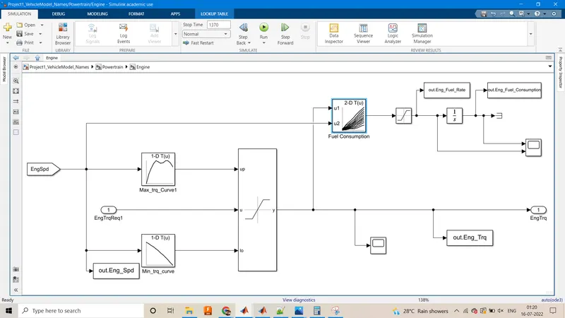
a. Engine Subsystem in Powertrain
1. For the Engine blocks we take the Engine required torque as the input
2. We use Engine speed from block to two 1-d lookup tables containing data for max and min torque curve, which is determined on the basis of Engine Map speed.
3. We then use saturation block to get the torque within specified limits and give that output to 2-d lookup table for fuel consumption rate.
4. The second input to the 2-d lookup table is taken as the Engine Speed.
5. The 2-d Fuel Consumption lookup table gives us the fuel consumption rate which we limit using saturation where lower limit is taken as 0.
6. We provide the fuel rate as input to an integrator block to get the fuel consumption rate.
7. We add to workspace blocks for Engine fuel rate, Engine fuel consumption, Engine torque & Engine speed to be used in Matlab.
8. The output of the subsystem is Engine torque.
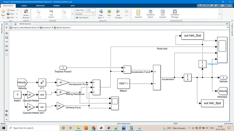
b. Vehicle Dynamics Block
1. Tractive force is the input to the subsystem.
2. We use from block for velocity variable while computing aerodynamic drag
3. We use formulae for Aerodynamic, rolling resistance & climbing force along with multiple gain blocks to get the respective forces.
4. Then we sum the above 3 forces and subtract that from the tractive force to get acceleration force
5. Divide the acceleration force with mass to get acceleration.
6. Subsequently integrate the acceleration to get velocity and distance.
7. The output of the subsystem is velocity.
8. We use to workspace blocks for distance & velocity.
UDDS Cycle:
We keep the switch in the initial file at position 1
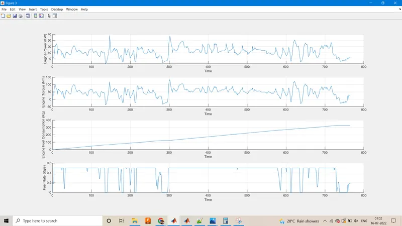
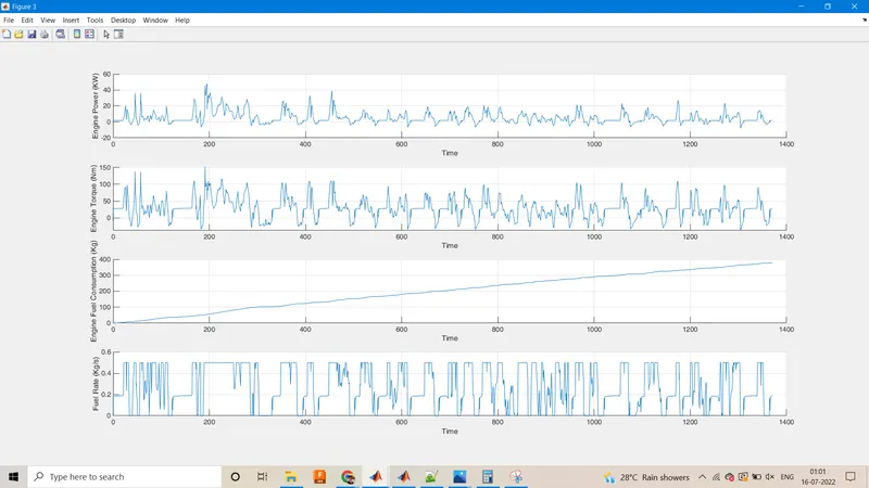
1. The Engine Power seems to be in direct proportion with the cycle and varies according to UDDS cycle.
2. Engine Torque is proportional to the cycle and varies in sync with the UDDS Drive cycle.
3. The Fuel Consumption varies linearly with time, i.e as time period increases fuel consumption also increses.
4. Fuel rate varies according to UDDS cycle with some flat notes due to the saturation provided in the model.
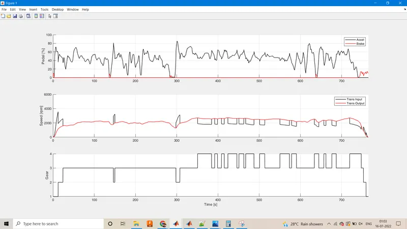
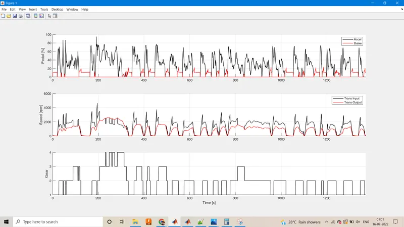
5. Acceleration varies with respect to the cycle.
6. Brake remains 0 when accelerating and has some value only when acceleration is 0.
7. Speed varies with respect to the cycle where output torque is always lesser than input torque (except when both are 0).
8. Gear command varies from 1 to 4 depending on the acceleration/braking required.
HWFET cycle:
We keep the switch in the initial file at position 2
1. The Engine Power seems to be in direct proportion with the cycle and varies according to HWFET cycle.
2. Engine Torque is proportional to the cycle and varies in sync with the HWFET Drive cycle.
3. The Fuel Consumption varies linearly with time, i.e as the time period increases fuel consumption also increases.
4. Fuel rate varies according to HWFET cycle with some flat notes due to the saturation provided in the model.
5. Acceleration varies with respect to the cycle.
6. Brake remains 0 when accelerating and has some value only when acceleration is 0.
7. Gear command varies from 1 to 4 depending on the acceleration/braking required.
%Intial file
%% Vehicle Parameters
M = 1500;       % Vehicle weight [kg]
Cr = 0.015;     % Rolling resistance coefficient
Rw = 0.35;      % Rolling radius [m]
Cd = 0.33;      % Drag coefficient
Af = 2;         % Frontal area [m2]
rhoa = 1.225;   % Air density [kg/m3]
Vwind = 0;      % Wind velocity [kmph]
g = 9.81;       % Gravitational acceleration [m/s2]
theta = 0;      % Slope [deg]
myu_road_tire = 1; % Coefficient of friction between tire - road interface

%% Powertrain Parameters
FDR = 3.73;                         % Final Drive Ratio / Diff Ratio
DiffEff = 0.99;                     % Differential efficiency (assumed independent of operating conditions)

NumGear = 4;                        % Number of gears in transmission
TransGear = [1:NumGear];            % Transmission Gears
TransRatio = [3.06, 1.62, 1, 0.7];  % Corresponding Transmission ratios
TransEff = 0.90;                    % Transmission efficiency (assumed independent of operating conditions)

TC_SR = [0, .5, .6, .7, .8, .87, .92, .94, .96, .97, 1];   % Torque Converter Speed Ratio (Matlab default) -> TurbSpd/PumpSpd
TC_TR = [2.232, 1.5462, 1.4058, 1.2746, 1.1528, 1.0732, 1.0192, 1, 1, 1, 1];   % Torque Converter Torque Ratio (Matlab default) -> TurbTrq/PumpTrq
TC_Cf = 1e-4 * [.72558, .66322, .63463, .59042, .51331, .4144, .29287, .22444, .12186, .04386, 0]; % Torque Converter Capacity Factor (Matlab default) -> PumpTrq/PumpSpd^2 [Nm/rpm^2]

load Vehicle_Data/Engine_data_1_9L_Saturn_95kW
load Vehicle_Data/Trans_Shift_map

%% Driver Parameters
Kp = 10;                    % P gain for driver PI model
Ki = 1;                     % I gain for driver PI model
Drive_Cycle_Select = 2;     % Drive cycle selection

% Drive cycle values in m/s

if Drive_Cycle_Select == 1
    load DriveCycles/UDDS;

elseif Drive_Cycle_Select == 2
    load DriveCycles/HWFET;

elseif Drive_Cycle_Select == 3
    load DriveCycles/FTP;

elseif Drive_Cycle_Select == 4
    load DriveCycles/US06;

elseif Drive_Cycle_Select == 5
    load DriveCycles/NEDC;

elseif Drive_Cycle_Select == 6
    load DriveCycles/WLTP;

end

time_end = cyc_time(end);
vel_end = cyc_vel(end);


%Processing File

%% Renaming variables
Time = out.tout;
Acc_Pdl = out.Acc_Pdl;          % Accelerator pedal [%]
Brk_Pdl = out.Brk_Pdl;          % Brake pedal [%]
Gear_Cmd = out.Gear_Cmd;        % Transmission gear
Trans_In_Spd = out.Trans_In_Spd*30/pi;  % Transmission input speed [rpm]
Trans_Out_Spd = out.Trans_Out_Spd*30/pi;% Transmission output speed [rpm]
Eng_Trq = out.Eng_Trq;          % Engine brake torque [Nm]
Eng_Spd = out.Eng_Spd*30/pi;    % Engine speed [rpm]
Eng_Fuel_Consump = out.Eng_Fuel_Consumption;    % Engine fuel consumption [g]
Veh_Dist = out.Veh_Dist/1000;   % Distance traveled by vehicle [km]
Veh_Spd = out.Veh_Spd*18/5;     % Vehicle speed [kmph]
Eng_Fuel_Rate=out.Eng_Fuel_Rate;

%% Data Analysis
Eng_Pwr = Eng_Spd*pi/30.*Eng_Trq/1000;   % Engine brake power [kW]
rho_petrol = 0.7197;                    % Density of petrol [kg/L]
kmpl = Veh_Dist(end)/(Eng_Fuel_Consump(end)/1000/rho_petrol);    % Fuel economy [kmpl]


%% Plotting vehicle characteristics time trace
figure()
subplot(3,1,1)
hold on
grid on
plot(Time, Acc_Pdl, 'linewidth', 1, 'Color', 'black');
plot(Time, Brk_Pdl, 'linewidth', 1, 'Color', 'red');
ylabel('Pedal [%]')
xlim([0, Time(end)]);
legend('Accel','Brake');
subplot(3,1,2)
hold on
grid on
plot(Time, Trans_In_Spd, 'linewidth', 1, 'Color', 'black');
plot(Time, Trans_Out_Spd, 'linewidth', 1, 'Color', 'red');
ylabel('Speed [rpm]')
xlim([0, Time(end)]);
ylim([0, 6000]);
legend('Trans Input','Trans Output');
subplot(3,1,3)
hold on
grid on
plot(Time, Gear_Cmd, 'linewidth', 1, 'Color', 'black');
xlim([0, Time(end)]);
xlabel('Time [s]');
ylabel('Gear');

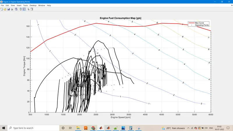
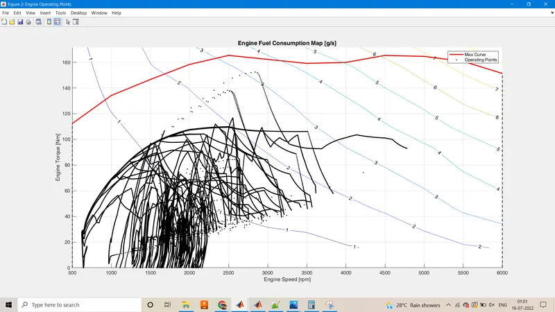
%% Plotting engine operating points on engine fuel map
figure('Name','Engine Operating Points');
hold on
grid on
title('Engine Operating Points','fontsize',12);
p1=plot(Eng_map_spd*30/pi,Eng_max_trq,'linewidth',2,'color','r');
p2=line([Eng_map_spd(end)*30/pi Eng_map_spd(end)*30/pi],[0 Eng_max_trq(end)]);
set(p2,'linewidth',1,'linestyle','--','color','k');
p3=line([Eng_map_spd(1)*30/pi Eng_map_spd(1)*30/pi],[0 Eng_max_trq(1)]);
set(p3,'linewidth',1,'linestyle','--','color','k');
[c,h] = contour(Eng_map_spd'*30/pi,Eng_map_trq,Eng_fuel_map');
clabel(c,h);
xlabel('Engine Speed [rpm]');
ylabel('Engine Torque [Nm]');
title('Engine Fuel Consumption Map [g/s]');
p4 = plot(Eng_Spd,Eng_Trq,'.','color','k');
legend([p1 p4],{'Max Curve','Operating Points'});
axis([Eng_map_spd(1)*30/pi Eng_map_spd(end)*30/pi 0 Eng_map_trq(end)]);


%Plotting Power, Torque, Fuel rate & fuel consumption wrt time
figure(3)
subplot(4,1,1)
hold on
grid on
plot(Time,Eng_Pwr)
xlabel("Time")
ylabel("Engine Power (KW)")
%Title("Engine Power Vs Time")

subplot(4,1,2)
hold on
grid on
plot(Time,Eng_Trq)
xlabel("Time")
ylabel("Engine Torque (Nm)")

subplot(4,1,3)
hold on
grid on
plot(Time,Eng_Fuel_Consump)
xlabel("Time")
ylabel("Engine Fuel Consumption (Kg)")

subplot(4,1,4)
hold on
grid on
plot(Time,Eng_Fuel_Rate)
xlabel("Time")
ylabel("Fuel Rate (Kg/s)")