Project 1

System Dynamics :-

It deals with modelling of multi domain systems through the use of a unified approach based on a ordinary differential & algebraicequation describing the static & dynamic effects.

Each systems has are two generalised variables -

1. Efforts :- generalised force ex. torque,force,voltage

2. Flow :- generalised flow/velocity. ex. velocity,current,mass flow

3. Power :- product of effort & flow variable.

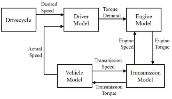
Model :-

Matlab Code :-

%%%%%%%%%%%%%%%%%%%%%%%%%%%%%%%%%%%%%%%%%%%%%%%%%%%%%%%%%%%%%%%%%%%%%
%% Skill-Lync -> Hybrid Drives Development
% Project 1 - Conventional Vehicle Model
% By - Chirag Bapna 

% Description:

%% Initialization File
% Initialization file for loading the variables for the Conventional vehicle simulation model

%% Vehicle Parameters
M = 1500;       % Vehicle weight [kg]
Cr = 0.015;     % Rolling resistance coefficient
Rw = 0.35;      % Rolling radius [m]
Cd = 0.33;      % Drag coefficient
Af = 2;         % Frontal area [m2]
rhoa = 1.225;   % Air density [kg/m3]
Vwind = 0;      % Wind velocity [kmph]
g = 9.81;       % Gravitational acceleration [m/s2]
theta = 0;      % Slope [deg]
myu_road_tire = 1; % Coefficient of friction between tire - road interface

%% Powertrain Parameters 
FDR = 3.73;                         % Final Drive Ratio / Diff Ratio
DiffEff = 0.99;                     % Differential efficiency (assumed independent of operating conditions)

NumGear = 4;                        % Number of gears in transmission
TransGear = [1:NumGear];            % Transmission Gears
TransRatio = [3.06, 1.62, 1, 0.7];  % Corresponding Transmission ratios
TransEff = 0.90;                    % Transmission efficiency (assumed independent of operating conditions)

TC_SR = [0, .5, .6, .7, .8, .87, .92, .94, .96, .97, 1];   % Torque Converter Speed Ratio (Matlab default) -> TurbSpd/PumpSpd  
TC_TR = [2.232, 1.5462, 1.4058, 1.2746, 1.1528, 1.0732, 1.0192, 1, 1, 1, 1];   % Torque Converter Torque Ratio (Matlab default) -> TurbTrq/PumpTrq
TC_Cf = 1e-4 * [.72558, .66322, .63463, .59042, .51331, .4144, .29287, .22444, .12186, .04386, 0]; % Torque Converter Capacity Factor (Matlab default) -> PumpTrq/PumpSpd^2 [Nm/rpm^2]

load Vehicle_Data/Engine_data_1_9L_Saturn_95kW
load Vehicle_Data/Trans_Shift_map

%% Driver Parameters
Kp = 10;                    % P gain for driver PI model
Ki = 1;                     % I gain for driver PI model
Drive_Cycle_Select = 1;     % Drive cycle selection

% Drive cycle values in m/s

if Drive_Cycle_Select == 1
    load DriveCycles/UDDS;
    
elseif Drive_Cycle_Select == 2
    load DriveCycles/HWFET;
    
elseif Drive_Cycle_Select == 3
    load DriveCycles/FTP;
    
elseif Drive_Cycle_Select == 4
    load DriveCycles/US06;
    
elseif Drive_Cycle_Select == 5
    load DriveCycles/NEDC;
    
elseif Drive_Cycle_Select == 6
    load DriveCycles/WLTP;
 
end

time_end = cyc_time(end);
vel_end = cyc_vel(end);

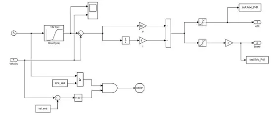
Driver Model:-

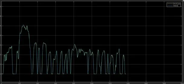
Graph :-

Control Model :-

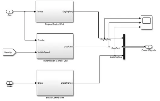
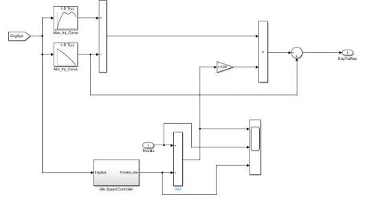
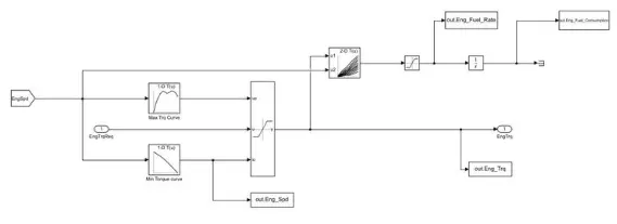
1. Engine Control Unit

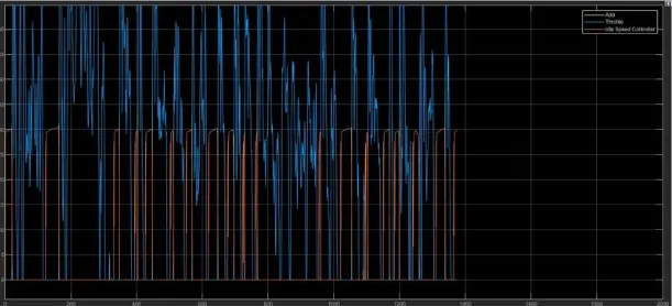
Graph :-

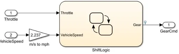
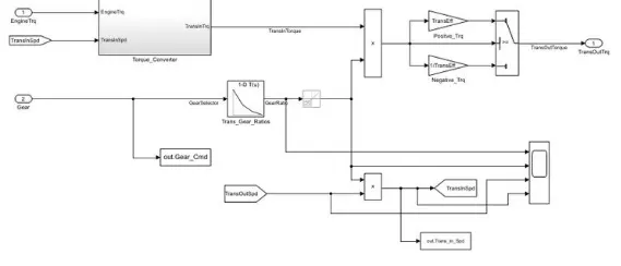
2.Transmission Control Unit :-

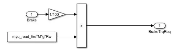
3. Brake Control Unit

Pwertrain :-

Engine :-

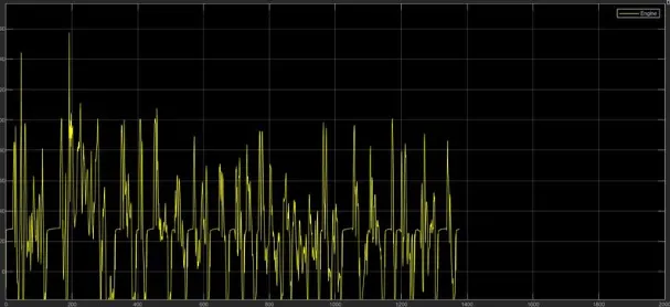
Graph:

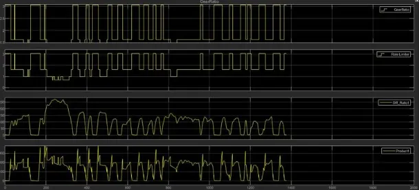
Transmission

Graph:

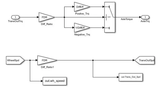
Differential :-

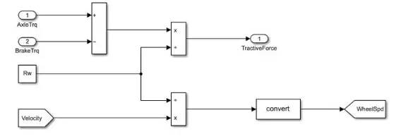
Wheels :

Vehicle Dynamics :

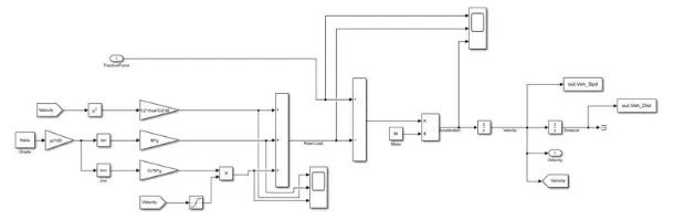
Graph :

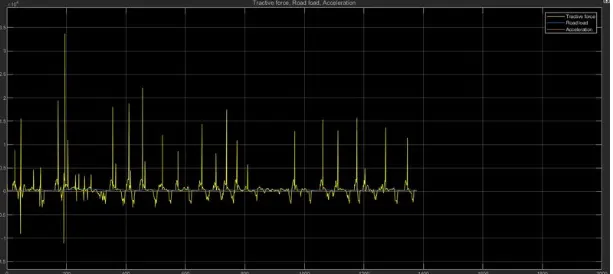
Fuel Economy :-

!. UDDS Cycle

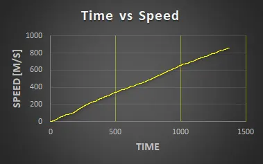
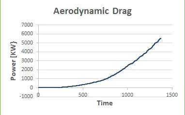
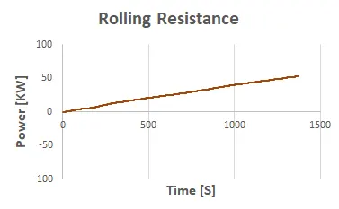
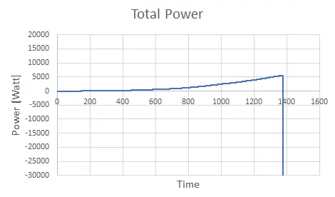
Conclusion :

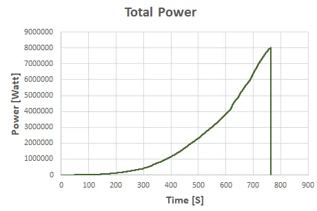
Total power gradually increases with increase in rolling resistance,drag & inertial resistance.

2.HWFET Cycle

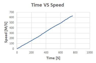
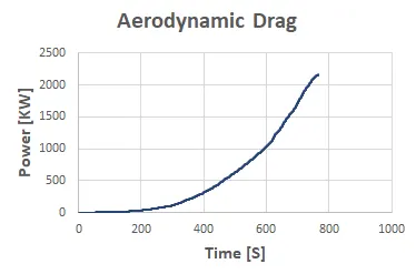
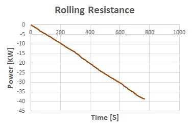
Conclusion :

Total power gradually increases with increase in rolling resistance,drag & inertial resistance but in this cycle impact is bad due to decrease in rolling resistance.

Result :

Comparing both the cycles we used UDDS cycle.

Plotting :

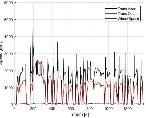
Transmission In & Out & wheel speed

Vehicle characteristics

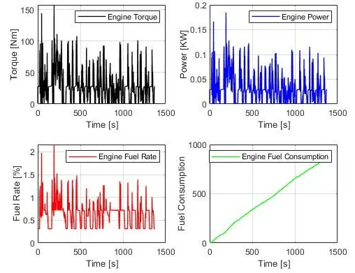
In this engine torque, power, fuel rate & fuel consumption increases wrt time.

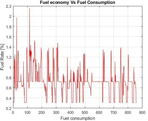
In this fuel consumption is suddenly increases as increase in fuel economy but if fuel economy is constant then fuel consumption is also constant.

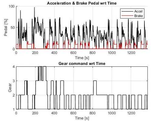
Accelerator pedal,brake pedal & gear command wrt time

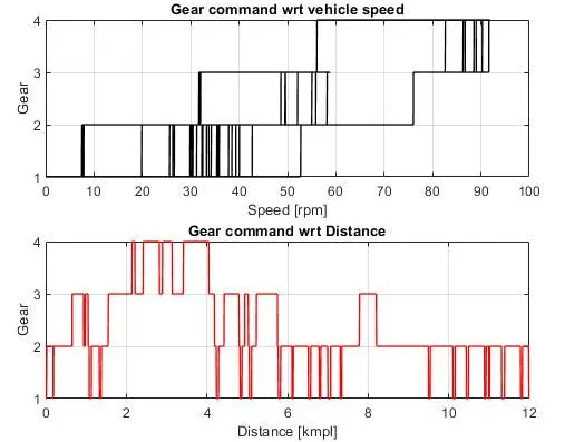
Gear command with actual speed

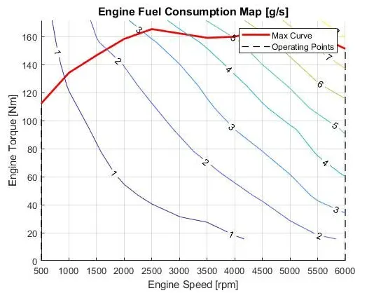
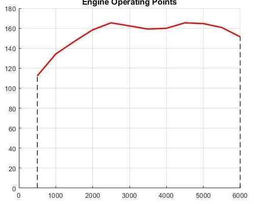
Engine operating points on engine fuel map

Engine Fuel Consumption Map