Project 1

TITLE – Development of Forward Energy Based Fuel Consumption Model of Conventional Vehicle.

AIM – The main aim of this project is to get familiar with the modelling process in Simulink, writing script in MATLAB, analyzing data and generating plots.

THEORY – A conventional vehicle uses an Internal Combustion Engine as power source which in turn uses fossil fuel (Petrol & Diesel) which contains up to 9000 Wh/kg of energy. Around the world the efficiency of Convention vehicle is around 20% to 35%. Efficiency is low due to Heat loss from Engine which is due to lower conversion ratio of Fuel Energy into Mechanical Energy there is also frictional losses in the Engine as well outside the Engine Like Transmission coupling, Gear box, Differential and other moving joints in vehicle.

Below images are made by me which will show a layout of Forward Model of Conventional Vehicle and how power flows from fuel to Wheels.

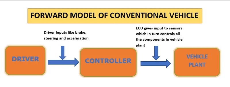
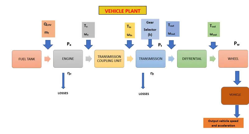
• Q_LHV – Calorific value/Lower Heating Value.
• T_e – Torque produced by engine.
• T_in – Torque input to the transmission.
• T_out – Torque output from the transmission and differential. m_f – Fuel mass flow rate.
• ω_e - Angular velocity or RPM produced by the engine.
• ω_in - Angular velocity or RPM produced by the engine serve as an input to transmission via coupling unit.
• ω_out – Angular velocity or RPM after getting transform by the transmission serves as input to differential and wheel.
• Gear selector (K) – It helps to get desire range of speed and torque at output for the given input of torque and speed.
• η_e – Engine efficiency.
• η_t – Transmission efficiency.
• P_e – Power of engine.
• P_t – Power of transmission.
• P_w – Power at wheels.

In this project a typical midsize car with 1.9 Liter and 4-speed automatic transmission is consider. Data is taken from ADVISOR data base developed by NREL, USA. Transmission shift map and controller is taken from MATLAB/Simulink example database.

The model in this project have capability to simulate on different Drive Cycle like UDDS, HWFET, FTP, NEDC & WLTP.

MATLAB SCRIPTS AND SIMULINK MODEL:

The below script is run to load all the variables in MATLAB workspace required to run the Simulink model and post processing work. Drive cycle selection is also done here in this script.

%%%%%%%%%%%%%%%%%%%%%%%%%%%%%%%%%%%%%%%%%%%%%%%%%%%%%%%%%%%%%%%%%%%%%
%% Skill-Lync -> Hybrid Drives Development
% Project 1 - Conventional Vehicle Model
% By - Ullekh Gambhira 

% Description:

%% Initialization File
% Initialization file for loading the variables for the Conventional vehicle simulation model


%% Vehicle Parameters
M = 1500;       % Vehicle weight [kg]
Cr = 0.015;     % Rolling resistance coefficient
Rw = 0.35;      % Rolling radius [m]
Cd = 0.33;      % Drag coefficient
Af = 2;         % Frontal area [m2]
rhoa = 1.225;   % Air density [kg/m3]
Vwind = 0;      % Wind velocity [kmph]
g = 9.81;       % Gravitational acceleration [m/s2]
theta = 0;      % Slope [deg]
myu_road_tire = 1; % Coefficient of friction between tire - road interface

%% Powertrain Parameters 
FDR = 3.73;                         % Final Drive Ratio / Diff Ratio
DiffEff = 0.99;                     % Differential efficiency (assumed independent of operating conditions)

NumGear = 4;                        % Number of gears in transmission
TransGear = [1:NumGear];            % Transmission Gears
TransRatio = [3.06, 1.62, 1, 0.7];  % Corresponding Transmission ratios
TransEff = 0.90;                    % Transmission efficiency (assumed independent of operating conditions)

TC_SR = [0, .5, .6, .7, .8, .87, .92, .94, .96, .97, 1];   % Torque Converter Speed Ratio (Matlab default) -> TurbSpd/PumpSpd  
TC_TR = [2.232, 1.5462, 1.4058, 1.2746, 1.1528, 1.0732, 1.0192, 1, 1, 1, 1];   % Torque Converter Torque Ratio (Matlab default) -> TurbTrq/PumpTrq
TC_Cf = 1e-4 * [.72558, .66322, .63463, .59042, .51331, .4144, .29287, .22444, .12186, .04386, 0]; % Torque Converter Capacity Factor (Matlab default) -> PumpTrq/PumpSpd^2 [Nm/rpm^2]

load Vehicle_Data/Engine_data_1_9L_Saturn_95kW
load Vehicle_Data/Trans_Shift_map

%% Driver Parameters
Kp = 10;                    % P gain for driver PI model
Ki = 1;                     % I gain for driver PI model
Drive_Cycle_Select = 1;     % Drive cycle selection

% Drive cycle values in m/s

if Drive_Cycle_Select == 1
    load DriveCycles/UDDS;
    
elseif Drive_Cycle_Select == 2
    load DriveCycles/HWFET;
    
elseif Drive_Cycle_Select == 3
    load DriveCycles/FTP;
    
elseif Drive_Cycle_Select == 4
    load DriveCycles/US06;
    
elseif Drive_Cycle_Select == 5
    load DriveCycles/NEDC;
    
elseif Drive_Cycle_Select == 6
    load DriveCycles/WLTP;
 
end

time_end = cyc_time(end);
vel_end = cyc_vel(end);

The Simulink Model:

Below are the screen shots of Simulink model in detail.

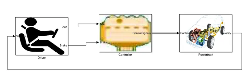
The Simulink model containing Driver block, Controller Block and Vehicle plant block. All the blocks will be shown below further.

Driver Block:

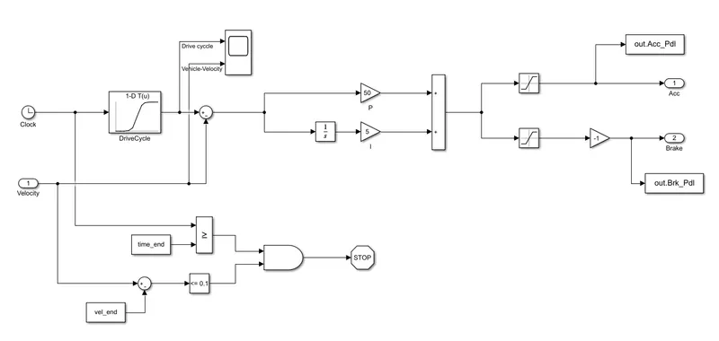
• It is an essential model using a PI controller.
• The logic of the PI controller is that it needs some error and based on that error it multiplies that with constant gain for p and for I it integrates the error and then multiplies with constant I. Then these 2 error values are added up. It serves as control command.
• Error is feed by the difference between the drive cycle speed and the speed of the vehicle that come s from vehicle dynamics. The input to drive cycle is time. The difference is error. If the difference is positive, positive signal is received by the command controller and if the error is negative then negative signal is received by the command controller after being processed by PI controller. The positive error tells that the driver is accelerating the vehicle and the negative error tell that the driver is applying brakes to the vehicle. The command control divides the signal into 2 part ) Acceleration 2.) Brake. These are 2 outputs from Driver Block.
• The lower Simulink Blocks are to stop the simulation.

Controller Block:

The controller Block is the Brain of the Vehicle as it interprets all the command from the drivers and decides and pass all the necessary signal to Powertrain Block.

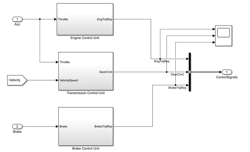
Input to the controller block is Acceleration demand from Driver Block which goes to Engine Control Unit Subsystem from this unit we get Engine Torque required by the vehicle, it also serves as input to Transmission Control unit along with Velocity as input. The Transmission control unit decides the gear command that is on which gear the vehicle is operating. Brake from the driver Block serves input to Brake Control Unit which gives output what is the brake torque required.

Powertrain Block:

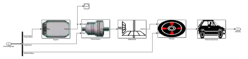
The powertrain block contains five subsystem that are Engine Block, Transmission Block, Differential Block, Wheel Block and Vehicle Dynamics Block.

All the Blocks are show below with explanation.

Engine Block:

Engine Block gives output of Fuel Rate, Engine Fuel Consumption in g/sec and Engine Torque.

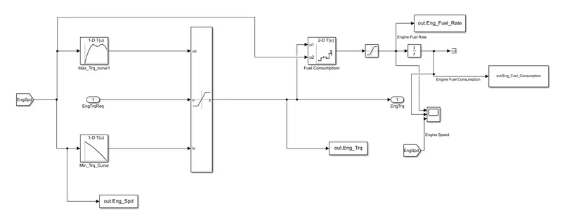
• Engine-Torque -Request come from the controller block.
• What does this model does is that based on the torque request from the controller checks whether the torque is between Max Torque curve1 or Minimum Torque curve, this is done by switching block which uses Engine torque request as threshold value basically the switch block saturates the torque base on Max and Min curve.
• It is also going take that Engine Torque and calculate fuel consumption using 2-D look up table where the data is already given for relation between Engine Torque and Fuel consumption.

Transmission Block:

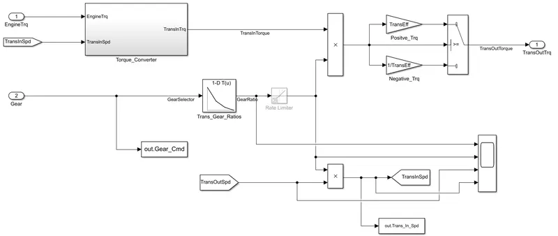
• It takes input the Engine torque from Engine Block, Gear input from gear selector from controller block.
• Using the gear selector, the gear ratio is defined.
• The gear ratio and transmission input Torque is multiplied.
• Then it gives the Transmission Out Torque after filtering the signal through logic whether the Torque is positive or negative using the Switch block which uses a threshold value zero (0) to decide.
• Transmission Out speed is back calculated from the Differential block or it is fetched from there which is multiplied by Gear ratio to get Transmission Input speed.
• Transmission Input speed serves as input to Torque converter subsystem along with Engine Torque. Torque converter subsystem gives Transmission Input Torque as output.

Differential Block:

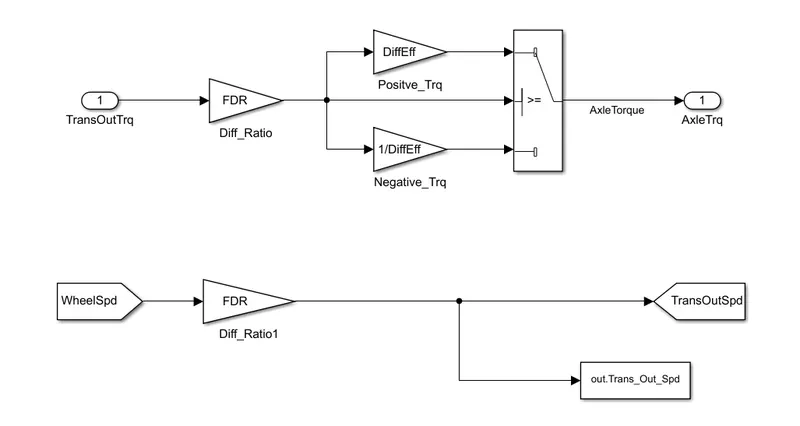
• Input to differential is the Transmission output Torque.
• Then there is going to be a final drive ratio, it is multiplied with transmission output Torque which will give axle Toque.
• Differential is going to have some efficiency; we are considering constant efficiency here. This efficiency will depend upon whether the Transmission out Torque is negative or positive torque.
• If the Transmission output Torque (TransOutTrq) is positive then it is multiplied with differential efficiency.
• If the Transmission output Torque (TransOutTrq) is negative then it will be divided differential efficiency. Negative torque is Torque coming from wheels.
• A switching block is used to switch between positive and negative torque. The threshold value over here is zero.
• Axle Torque is the output of this Block.

Wheel Block:

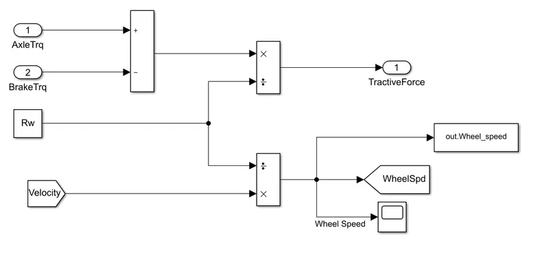
• Axle Torque serves as input to the wheels.
• Brake Torque input is going to retard the wheels.
• So, the subtract block will subtract Axle Torque & Brake Torque and give the net axle torque which is the wheel torque.
• The wheel torque will be divided by the Rolling Radius of the wheel which will give Tractive force assuming no loss of traction.
• Velocity Block is coming form vehicle dynamics block it is divided by Rolling Radius of the wheel which will give angular velocity of the wheels which is equal to wheel speed.

Vehicle Dynamics Block:

The below Equation is used to model the Vehicle dynamics block.

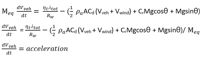
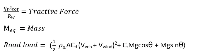
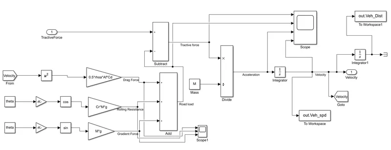
• Tractive force is input to Vehicle Dynamics Block and it subtracted by Road Load.
• Road load is calculated using Constant blocks Gain blocks and the added together using Add Block.
• The tractive force calculated is divide by mass as shown in the equation which will give Acceleration.
• After Integrating the acceleration using Integrator block, we get velocity.
• Velocity signal is further converted to distance using Integrator Block.
• To workspace blocks are used to send vehicle speed and distance to workspace.

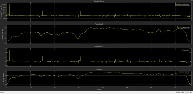
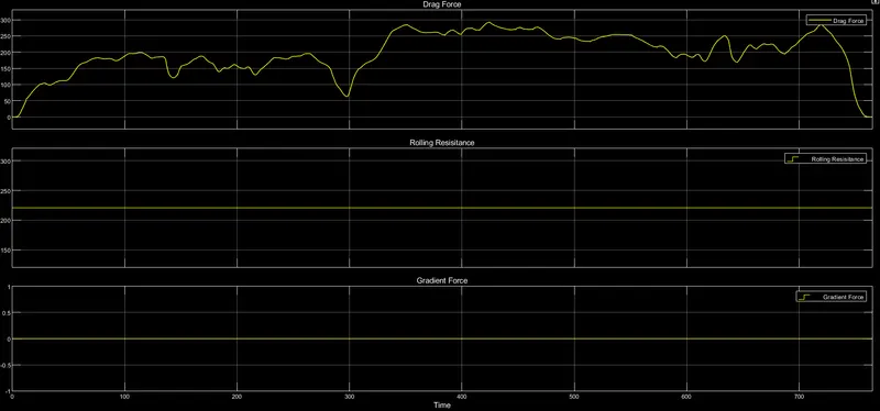
After running the Simulink Model, we obtain certain graphs through scope blocks. Below are the Screenshot of some observation.

FOR UDDS DRIVE CYCLE:

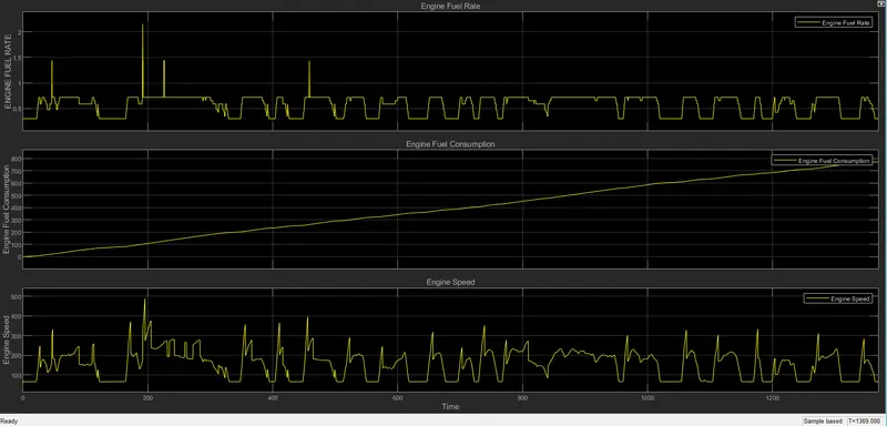
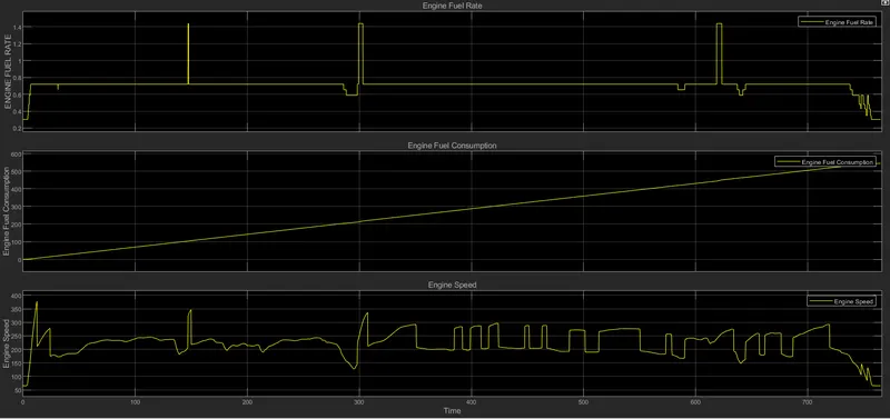
The above graph show Engine Fuel Rate, Engine Fuel Consumption in g/s and Engine Speed

• From the First Graph we can observe that Engine fuel rate spikes up when when more speed is demanded by the driver it directly resembles Engine speed. when ever Engine speed spikes Fuel Rate spikes up.
• The Engine Fuel consumption increase almost linearly

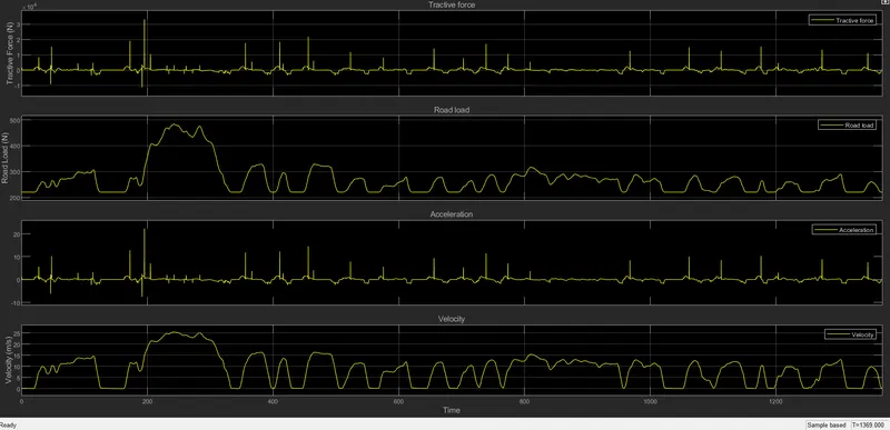
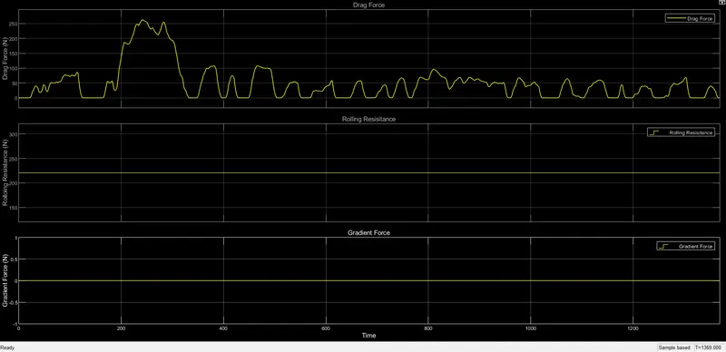
FOR HWFET DRIVE CYCLE:

After running the Simulink Model, we will run the processing script in the MATLAB to analyse the data obtain from the simulation of the model. The script has been modified to generate certain plots. Below is the script.

%%%%%%%%%%%%%%%%%%%%%%%%%%%%%%%%%%%%%%%%%%%%%%%%%%%%%%%%%%%%%%%%%%%%%
%% Skill-Lync -> Hybrid Drives Development
% Project 1 - Conventional Vehicle Model
% By - Ullekh Gambhira 

% Description:
% The following file is to used with the Initialization file and Simulink
% results for post-processing of the data.
% The file is incomplete, has some examples of how the data is imported
% into a readable format, data analysis and plotting examples.
% Based on the project task, use commands in a similar format as given
% below, to analyse the data and generate required plots.
% You can change variable names if desired

%% Post-Processing File
%  File for post-processing the Conventional vehicle simulation model data

%% Renaming variables
Time = out.tout;
Acc_Pdl = out.Acc_Pdl;          % Accelerator pedal [%]
Brk_Pdl = out.Brk_Pdl;          % Brake pedal [%]
Gear_Cmd = out.Gear_Cmd;        % Transmission gear
Trans_In_Spd = out.Trans_In_Spd*30/pi;  % Transmission input speed [rpm]
Trans_Out_Spd = out.Trans_Out_Spd*30/pi;% Transmission output speed [rpm]
Eng_Trq = out.Eng_Trq;          % Engine brake torque [Nm]
Eng_Spd = out.Eng_Spd*30/pi;    % Engine speed [rpm]
Eng_Fuel_Consump = out.Eng_Fuel_Consumption;    % Engine fuel consumption [g]
Eng_Fuel_Rate = out.Eng_Fuel_Rate; % Engine fuel rate
Veh_Dist = out.Veh_Dist/1000;   % Distance traveled by vehicle [km]
Veh_Spd = out.Veh_spd*18/5;     % Vehicle speed [kmph]
wheel_speed = out.Wheel_speed; % Wheel speed

%% Data Analysis
Eng_Pwr = Eng_Spd*pi/30*Eng_Trq/1000;   % Engine brake power [kW]
rho_petrol = 0.7197;                    % Density of petrol [kg/L]
kmpl = Veh_Dist(end)/(Eng_Fuel_Consump(end)/1000/rho_petrol);    % Fuel economy [kmpl] 



%% Plotting vehicle characteristics time trace
figure(1)
subplot(3,1,1)
hold on
grid on
plot(Time, Acc_Pdl, 'linewidth', 1, 'Color', 'black');
plot(Time, Brk_Pdl, 'linewidth', 1, 'Color', 'red');
ylabel('Pedal [%]')
xlim([0, Time(end)]);
legend('Accel','Brake');
subplot(3,1,2)
hold on
grid on
plot(Time, Trans_In_Spd, 'linewidth', 1, 'Color', 'black');
plot(Time, Trans_Out_Spd, 'linewidth', 1, 'Color', 'red');
ylabel('Speed [rpm]')
xlim([0, Time(end)]);
ylim([0, 6000]);
legend('Trans Input','Trans Output');
subplot(3,1,3)
hold on
grid on
plot(Time, Gear_Cmd, 'linewidth', 1, 'Color', 'black');
xlim([0, Time(end)]);
xlabel('Time [s]');
ylabel('Gear');

figure(2)
hold on
grid on
plot(Time, Eng_Fuel_Consump.Data, 'linewidth', 1, 'Color', 'black');
plot(Time, Eng_Fuel_Rate.Data, 'linewidth', 1, 'Color', 'red');
xlabel('Fuel consumption')
ylabel('Fuel Rate')
xlim([0, Time(end)]);
legend('fuel consumption','Fuel Rtae');

figure(3)
hold on
grid on
plot(Time, Eng_Spd.Data, 'linewidth', 1, 'Color', 'g');
plot(Time, Trans_In_Spd, 'linewidth', 1, 'Color', 'blue');
plot(Time, Trans_Out_Spd, 'linewidth', 1, 'Color', 'red');
plot(Time, wheel_speed.Data, 'linewidth', 1, 'Color', 'yellow');
xlabel('Time')
ylabel('Speed')
xlim([0, Time(end)]);
legend('Engine_Speed','Trans_In_Speed','Trans_Out_Speed','wheel_speed');

% Plotting Engine Torue, power, Fuel Rtae, Fuel Consumption
figure(4)
subplot(2,2,1)
plot(Time, Eng_Trq.Data, 'linewidth', 1, 'Color', 'green');
xlabel('Time')
ylabel('Torque [NM]')
legend('Torque');

subplot(2,2,2)
plot(Time, Eng_Pwr.Data, 'linewidth', 1, 'Color', 'black');
xlabel('Time')
ylabel('Power [KW]')
legend('POWER');

subplot(2,2,3)
plot(Time, Eng_Fuel_Rate.Data, 'linewidth', 1, 'Color', 'red');
xlabel('Time')
ylabel('Fuel Rtae')
legend('Fuel Rate');

subplot(2,2,4)
plot(Time, Eng_Fuel_Consump.Data, 'linewidth', 1, 'Color', 'blue');
xlabel('Time')
ylabel('Fuel consumption in KMPL')
legend('Fuel consumption');


%% Plotting engine operating points on engine fuel map
figure('Name','Engine Operating Points');
hold on
grid on
title('Engine Operating Points','fontsize',12);
p1=plot(Eng_map_spd*30/pi,Eng_max_trq,'linewidth',2,'color','r');
p2=line([Eng_map_spd(end)*30/pi Eng_map_spd(end)*30/pi],[0 Eng_max_trq(end)]);
set(p2,'linewidth',1,'linestyle','--','color','k');
p3=line([Eng_map_spd(1)*30/pi Eng_map_spd(1)*30/pi],[0 Eng_max_trq(1)]);
set(p3,'linewidth',1,'linestyle','--','color','k');
[c,h] = contour(Eng_map_spd'*30/pi,Eng_map_trq,Eng_fuel_map');
clabel(c,h);
xlabel('Engine Speed [rpm]');
ylabel('Engine Torque [Nm]');
title('Engine Fuel Consumption Map [g/s]');
%a = plot(Eng_Spd,Eng_Trq);
%legend([p1 p4],{'Max Curve','Operating Points'});
%axis([Eng_map_spd(1)*30/pi Eng_map_spd(end)*30/pi 0 Eng_map_trq(end)]);

OBSERVATIONS:

FOR UDDS DRIVE CYCLE:

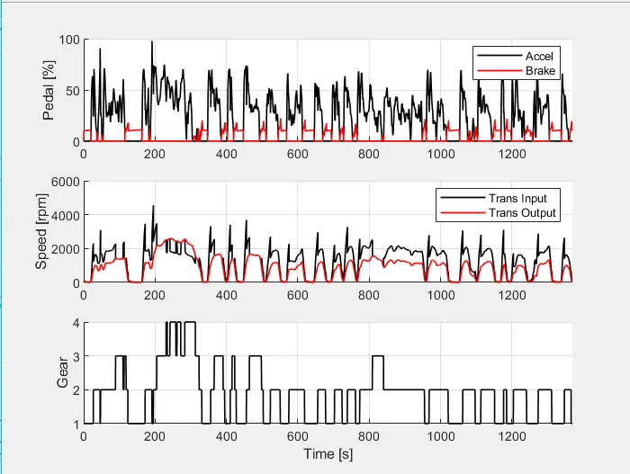
The above graph shows

• Acceleration and Brake demand from the driver. Where the acceleration is always more than the Brake which is good for fuel economy. The unit is percentage.
• The 2^nd graph shows Transmission Input speed and Transmission Output Speed. The maximum Transmission Input speed is above 4000 Rpm corresponding to it the Transmission Output Speed is less and it less through the simulation because it is a UDDS cycle.
• The 3^rd graph shows the gear number or the gear that vehicle is currently in. Maximum time the vehicle is in 2^nd

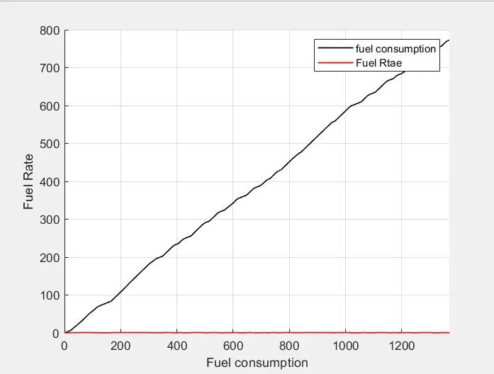
The above graph shows

• Fuel rate in red colour it can be observe that it is corresponding to zero cause from below graph we observe that the peak fuel rate is 2 g/sec.
• The Fuel consumption increases with time in a linear way. Here the simulation time is 1369 seconds for UDDS cycle.

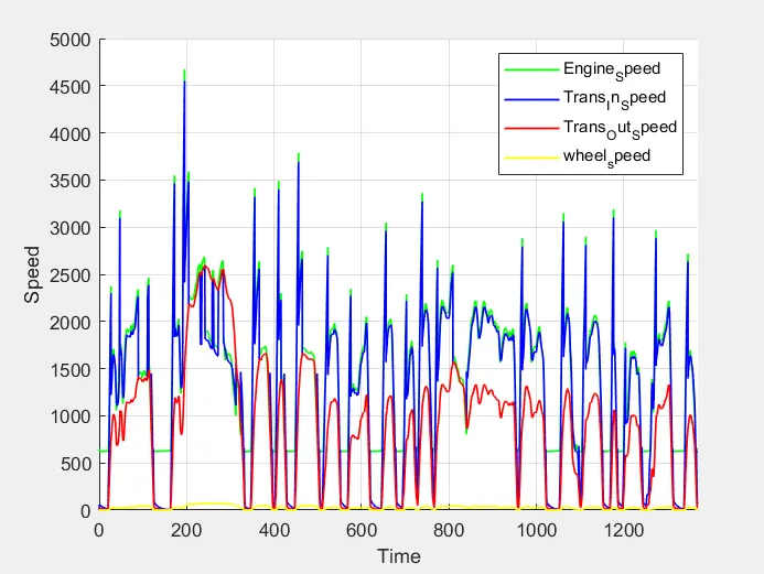
The above graph compares Engine Speed in green colour, Transmission Input speed in blue colour, Transmission output speed in red colour and Wheel speed in yellow colour.

• Engine Speed is lower or equal to Transmission Input speed but greater than Transmission output speed and Wheel speed.
• Transmission Input speed is always greater than Transmission output speed and Wheel speed.
• Transmission output speed is always less than Transmission Input speed because this is UDDS drive cycle and vehicle move in less speed.
• The wheel speed is always less the all the speed in the above graph.

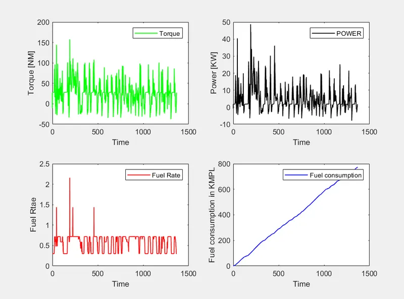
In the above graph we can see four different graphs of Torque, power, Fuel rate and Fuel consumption.

• The torque graph helps to observe the maximum torque that the vehicle will require for UDDS drive cycle. It also shows the negative torque. Altogether it will help to design efficient and economical Powertrain.
• The Power graphs helps to understand what is the maximum power for UDDS drive cycle in this case it is around 50 Kw. It also shows the negative power. Which will again altogether will help to design efficient and economical Powertrain.
• The Fuel rate graph shows what is the average fuel rate through the cycle the maximum over here is 2 g/sec and average is around less than 1.
• The Engine Fuel consumption increase almost linearly with time till the end of drive cycle cause with increase in time power demand increases.

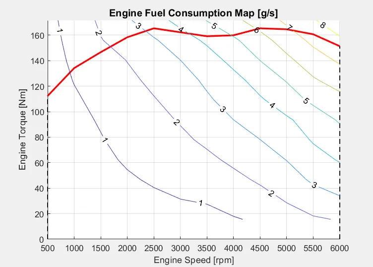
The above graph shows Engine Fuel consumption where the contour lines number denotes fuel consumption in g/sec and we can map out what is the fuel consumption for particular Engine Speed and Engine Torque by tracing the red line. For example, the fuel consumption at 160 Nm and 2500 Rpm is 3 g/sec.

FOR HWFET DRIVE CYCLE:

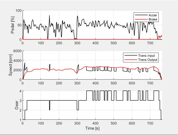
The above graph shows

• Acceleration and Brake demand from the driver. Where the acceleration is always more than the Brake which is good for fuel economy. The unit is percentage. The brake demand is very less cause it is HWFET cycle.
• The 2^nd graph shows Transmission Input speed and Transmission Output Speed. The maximum Transmission Input speed is below 4000 Rpm corresponding to it the Transmission Output Speed is less but maximum time the Transmission Output Speed is more than Transmission Input speed in HWFET cycle.
• The 3^rd graph shows the gear number or the gear that vehicle is currently in. Maximum time the vehicle is in 4^th

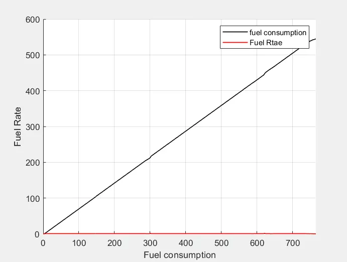
The above graph shows

• Fuel rate in red colour it can be observe that it is corresponding to zero cause from below graph we observe that the peak fuel rate is below 1.5 g/sec.
• The Fuel consumption increases with time in a linear way. Here the simulation time is 765 seconds for HWFET cycle.

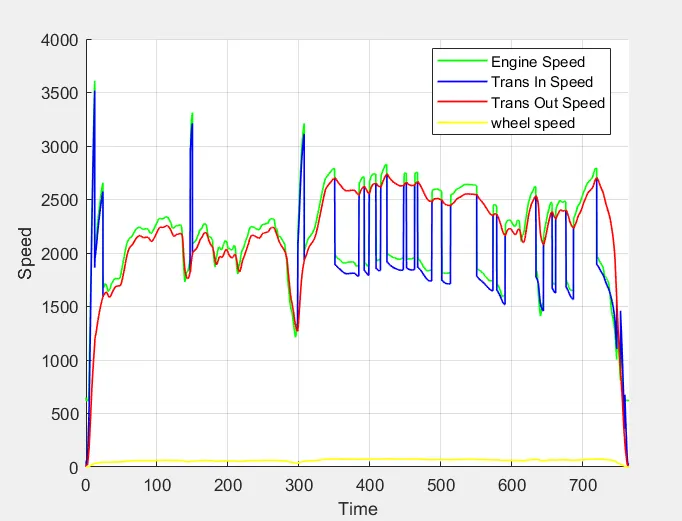
The above graph compares Engine Speed in green colour, Transmission Input speed in blue colour, Transmission output speed in red colour and Wheel speed in yellow colour.

• Engine Speed is lower or equal or sometimes even higher than Transmission Input speed but greater than Transmission output speed and Wheel speed.
• In HWFET cycle Transmission Input speed is greater than Transmission output speed only for lower gear ratio but maximum time in this cycle Transmission output speed is greater than Transmission Input speed because the vehicle propels at higher gear ratio on Highways.
• The wheel speed is always less the all the speed in the above graph.

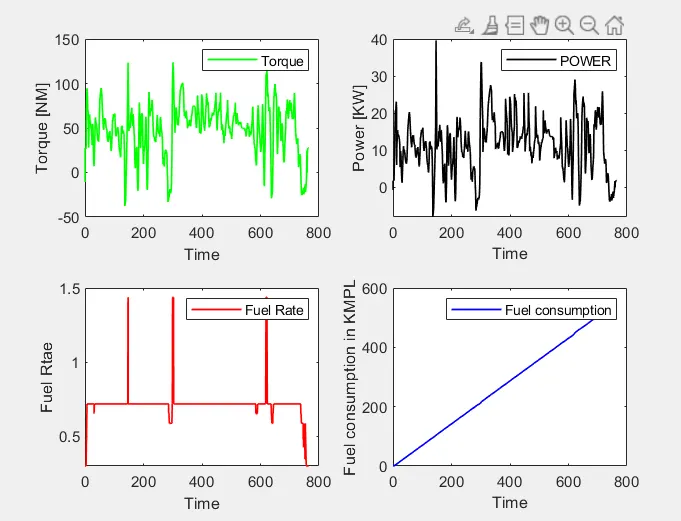
In the above graph we can see four different graphs of Torque, power, Fuel rate and Fuel consumption.

• The torque graph helps to observe the maximum torque that the vehicle will require for HWFET drive cycle. It also shows the negative torque. Altogether it will help to design efficient and economical Powertrain. The torque require is less than UDDS cycle.
• The Power graphs helps to understand what is the maximum power for HWFET drive cycle in this case it is around 40 Kw. It also shows the negative power. Which will again altogether will help to design efficient and economical Powertrain. The power require is less than UDDS drive Cycle.
• The Fuel rate graph shows what is the average fuel rate through the cycle the maximum over here is less than 1.5 g/sec and average is around less than 1.
• The Engine Fuel consumption increase almost linearly with time till the end of drive cycle cause with increase in time power demand increases.

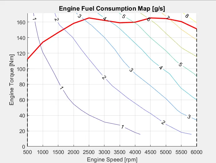
The above graph shows Engine Fuel consumption where the contour lines number denotes fuel consumption in g/sec and we can map out what is the fuel consumption for particular Engine Speed and Engine Torque by tracing the red line. For example, the fuel consumption at 160 Nm and 2500 Rpm is 3 g/sec.