Project 1
we are to make a forward energy model of a conventional fuel consumed vehicle.
The main goal of this project is to get familiar with the modeling process, writing scripts in Matlab, modeling in Simulink, analyzing data and generating plots.
In this project, a typical midsize car with a 1.9L engine and a 4-speed automatic transmission is considered. Data is taken from ADVISOR data base developed by NREL, USA. Transmission shift map and controller is taken from Matlab/Simulink example database.The model developed has the capability to simulate the vehicle on different drive cycles like UDDS, HWFET, FTP, NEDC, etc.
we are to use the given data of the matlab scripting provided for the simulink model and the model blocks provided for the vehicle.
the model block consist of ‘Driver’ block, which is a basic PI controller that generates accelerator and brake pedal outputs to match the desired and actual vehicle speeds. The ‘Controller’ block is the brains of the vehicle, representing the electronic controls units. Based on the driver inputs, it generates desired engine torque, desired transmission gear and desired brake torque. These inputs are fed to the ‘Powertrain’ block which represents the drivetrain of the vehicle.
the drive train or the power train consist of the major components of a vehicle system they are:
It consists of an ‘Engine’ connected to the ‘Automatic Transmission’ through a ‘Torque
Converter’. The output of the transmission is connected to the ’Differential’, which powers the ‘Wheels’, that provides the tractive force for vehicle acceleration. The longitudinal dynamics of the vehicle along with the road load is represented in the ‘Vehicle Dynamics’ block.
after once we simulate the block model with the missing blocks we are to take in a matlab code that is given by the questioner, it is called “Project1_ProcessingFile.m” it is the Matlab script used to analyze this data and to generate plots.
To do list:
1) Load the Project1 folder as the Current Folder in Matlab.
2) Run the “Project1_InitFile.m” Matlab script.
3) The provided vehicle Simulink model “Project1_VehicleModel.slx” is incomplete. The engine and vehicle dynamics block contents have been deleted. Build the Simulink blocks by referring to the course lecture and example block images provided. You can run the model and analyze the results using a ‘Scope’ for debugging.
4) Add additional ‘To Workspace’ blocks for transferring the desired Simulink vehicle data into the Matlab workspace.
5) Modify the “Project1_ProcessingFile.m” as per the desired plots and required calculations.
To make post processing of the data to find:
a. Tabulate the fuel economy numbers (kmpl) for UDDS and HWFET cycle. This forms the baseline numbers for comparing with the future hybrid version.
b. Plot the time trace for engine, transmission input, transmission output and wheel speed on one plot.
c. Plot engine torque, engine power, fuel rate and fuel consumption using subplots.
d. Plot accelerator and brake pedal, gear command, vehicle desired and actual speed, vehicle distance using subplots.
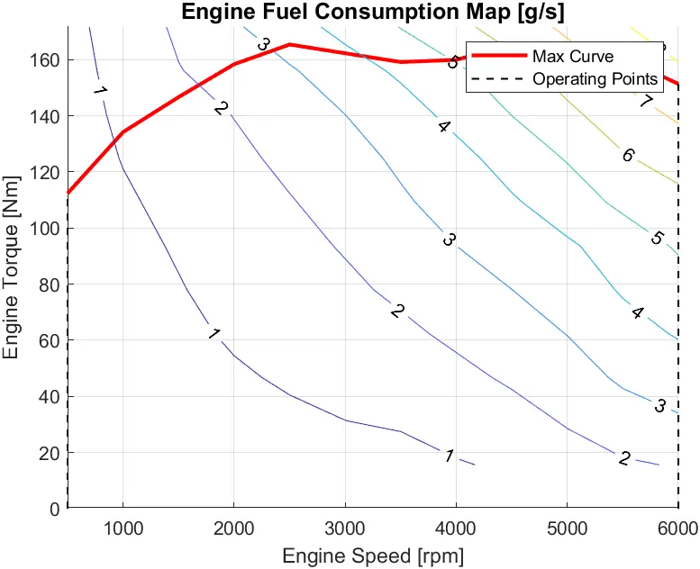
e. Plot the engine operating points on the engine fuel map.
f. Write down appropriate brief comments on each of these plots, describing the vehicle behavior throughout the drive cycle.
g. Generate the plots for both drive cycles
we are to make a model of the conventional vehicle and test it with the drive cycle data
we are to check for UDDC and HWFET cycle
first we need to run the matlab code called “Project1_InitFile.m”, this data is provided and we are taking it into the matlab environment to make the model simulation with its basic inputs.
FIRST CODE INPUT:
clear all
close all
clc
%%%%%%%%%%%%%%%%%%%%%%%%%%%%%%%%%%%%%%%%%%%%%%%%%%%%%%%%%%%%%%%%%%%%%
%% Skill-Lync -> Hybrid Drives Development
% Project 1 - Conventional Vehicle Model
% By - Sikkandar faiz

% Description:

%% Initialization File
% Initialization file for loading the variables for the Conventional vehicle simulation model

%% Vehicle Parameters
M = 1500;       % Vehicle weight [kg]
Cr = 0.015;     % Rolling resistance coefficient
Rw = 0.35;      % Rolling radius [m]
Cd = 0.33;      % Drag coefficient
Af = 2;         % Frontal area [m2]
rhoa = 1.225;   % Air density [kg/m3]
Vwind = 0;      % Wind velocity [kmph]
g = 9.81;       % Gravitational acceleration [m/s2]
theta = 0;      % Slope [deg]
myu_road_tire = 1; % Coefficient of friction between tire - road interface

%% Powertrain Parameters
FDR = 3.73;                         % Final Drive Ratio / Diff Ratio
DiffEff = 0.99;                     % Differential efficiency (assumed independent of operating conditions)

NumGear = 4;                        % Number of gears in transmission
TransGear = [1:NumGear];            % Transmission Gears
TransRatio = [3.06, 1.62, 1, 0.7];  % Corresponding Transmission ratios
TransEff = 0.90;                    % Transmission efficiency (assumed independent of operating conditions)

TC_SR = [0, .5, .6, .7, .8, .87, .92, .94, .96, .97, 1];   % Torque Converter Speed Ratio (Matlab default) -> TurbSpd/PumpSpd
TC_TR = [2.232, 1.5462, 1.4058, 1.2746, 1.1528, 1.0732, 1.0192, 1, 1, 1, 1];   % Torque Converter Torque Ratio (Matlab default) -> TurbTrq/PumpTrq
TC_Cf = 1e-4 * [.72558, .66322, .63463, .59042, .51331, .4144, .29287, .22444, .12186, .04386, 0]; % Torque Converter Capacity Factor (Matlab default) -> PumpTrq/PumpSpd^2 [Nm/rpm^2]

load Vehicle_Data/Engine_data_1_9L_Saturn_95kW
load Vehicle_Data/Trans_Shift_map

%% Driver Parameters
Kp = 10;                    % P gain for driver PI model
Ki = 1;                     % I gain for driver PI model
Drive_Cycle_Select = 1;     % Drive cycle selection

% Drive cycle values in m/s

if Drive_Cycle_Select == 1
    load DriveCycles/UDDS;

elseif Drive_Cycle_Select == 2
    load DriveCycles/HWFET;

elseif Drive_Cycle_Select == 3
    load DriveCycles/FTP;

elseif Drive_Cycle_Select == 4
    load DriveCycles/US06;

elseif Drive_Cycle_Select == 5
    load DriveCycles/NEDC;

elseif Drive_Cycle_Select == 6
    load DriveCycles/WLTP;

end

time_end = cyc_time(end);
vel_end = cyc_vel(end);
this data input contains the basic required inputs like the vehicle parameters, power train parameters and thedrive cycle selection parameters for the model simulation.
then take in the simulink model into the system.
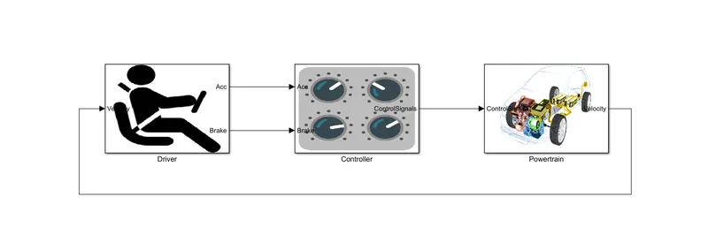
these forms the basic units of a vehicle system. the easy block representation is given below for better understanding
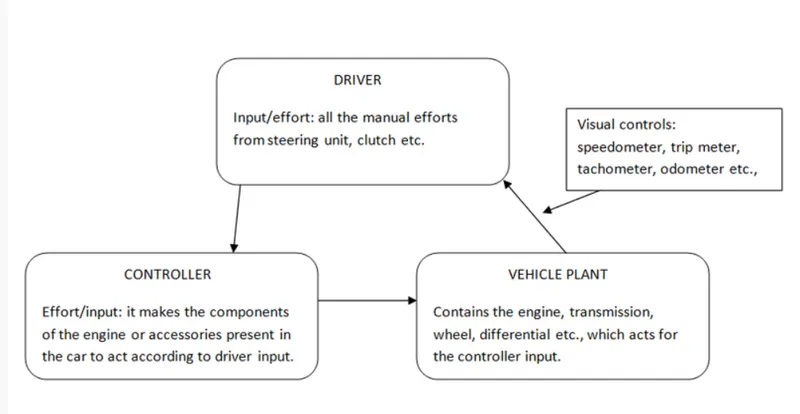
the first representation of the vehicle system is but the driver, who is responsible for the physical inputs such as acceleration, brake, clutch, steering control, gear shifting, etc., according to which the system takes in the input and sends it to the control unit.
the control unit then sends on the input signals from the driver to the vehicles respective components to get a required outcome.
the vehicle unit or power train contains the major components that make up an automobile which are engine, transmission control, transmission, differentials, fuel tank, wheels etc., the components react to the inputs received from the control unit. From the vehicle plant some of the visual controls are sent back to the driver for understanding if the working of vehicle system is as the given input. the vehicle plant block components are given below.
the simulink model runs with the help of first code tookin. we can select the cycle we are to find data in the first code by making few changes to it. in the drive cycle select we can make those changes.1 for UDDC, 2 HWFET, 3 FTP, 4 US06, 5 NEDC, 6 WLTP.
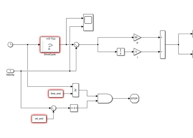
before taking in the code the model will be incomplete without few input variables so it is mandatory to run the “Project1_InitFile.m” script. if the model is opened without the code we can find the models as such red border as below.
once done we can start with the basic components of the model blocks.
DRIVER BLOCK:
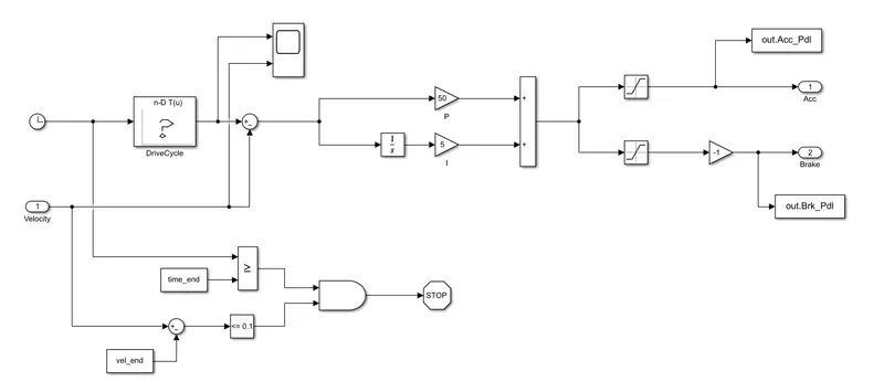
it contains the physical inputs from the driver like acceleration, brake, clutch, steering control, gear shifting, etc., according to which the system takes in the input and sends it to the control unit.
the PI controller checks the changes between the required drive cycle and the vehicle speed by providing outputs such as acceleration and brake pedal.
CONTROLLER MODEL:
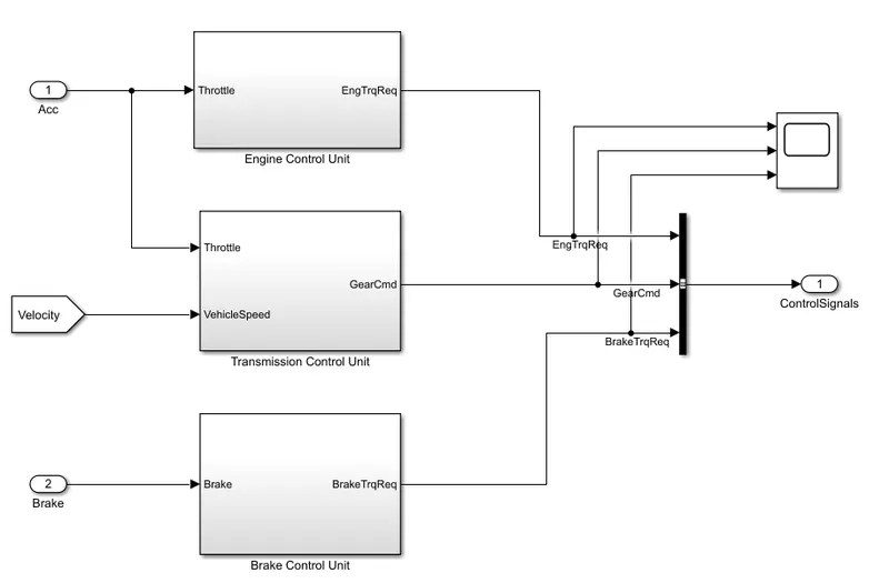
according to the driver input the controller makes the vehicle components to act accordingly. it seems as the main brain of the vehicle system. after taking in the needed driver inputs the controller understands the required output that has to begiven to the power train.
ENGINE CONTROL UNIT:
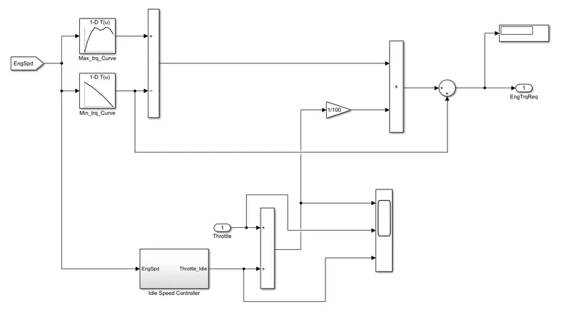
compares the max and min torque and gives out the actual required torque. the throttle input adds on witht the idle speed controller to provide the required torque.
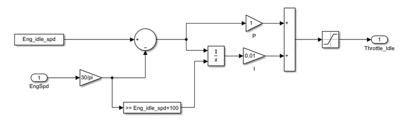
IDLE SPEED CONTROLLER:
TRANSMISSION CONTROL:
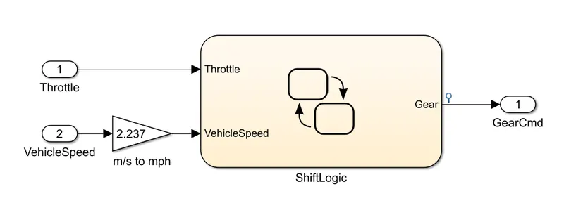
this block controls the gear shifting for the vehicle with help of a chart.
SHIFT LOGIC:
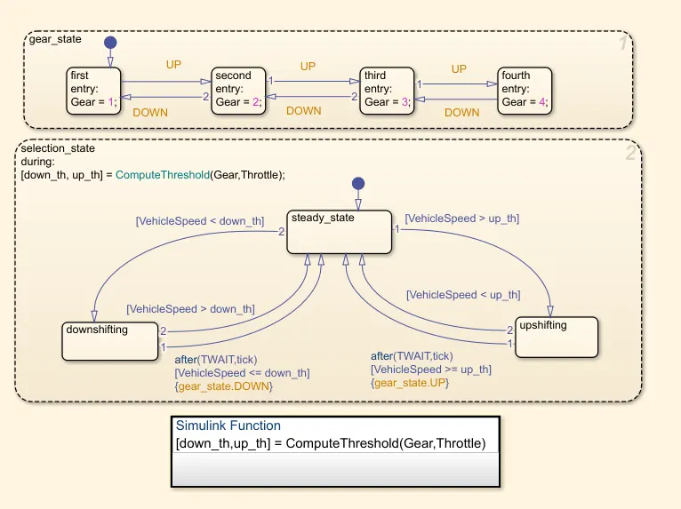
the gear shifting is done with the help of this chart which takes in the inputs such as throttle response and the vehicle speed and makes the gear shift according to them.
BRAKE CONTROL UNIT:
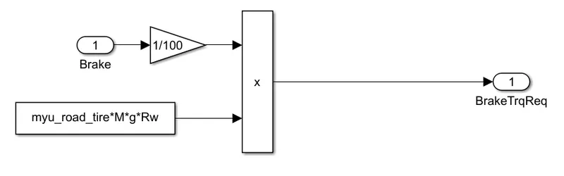
it outputs the required brake torque according to the given brake pedal value and the value is sent to the wheel unit.
POWER TRAIN MODEL:
it contains the major operating systems of an automobile like engine, transmission, wheels etc.,
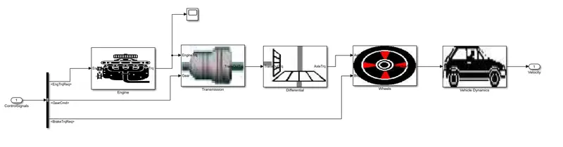
it takes in the pre informations from the driver and controller block and sends it to the engine and then onto the transmission and so on.
ENGINE MODEL:
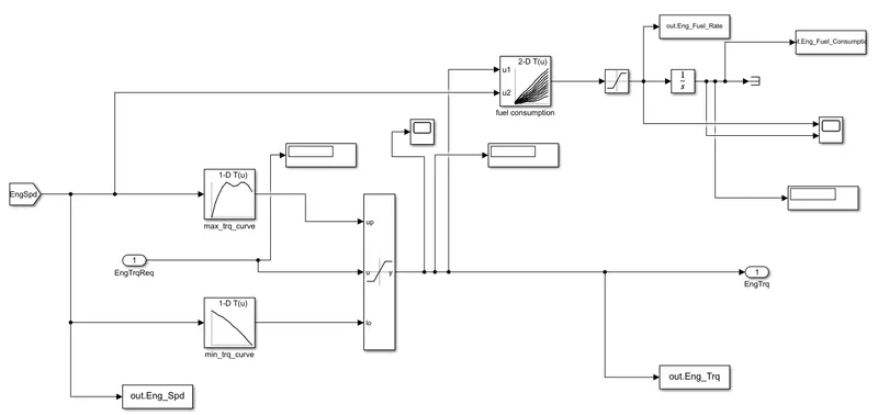
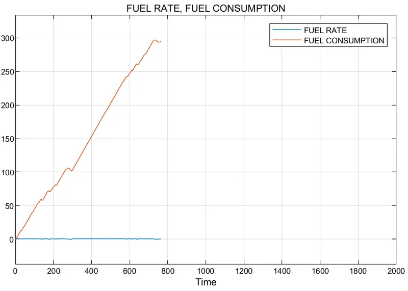
the values from the controller block is taken in and the torques like max and min are made into engine torque and the fuel rate and consumption are made as output.
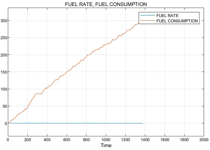
the look up table is helpful in mapping the fuel consumption of the engine and is found by integrating the value of fuel rate.
the data from the engine block is taken to the matlab workspace for post processing.
scope is attached to the fuel rate and consumption, to understand the change in them.
TRANSMISSION MODEL:
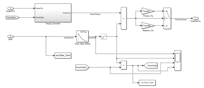
it is a representation of an automatic transmission. it sends data to the differential unit.
TORQUE CONVERTER:
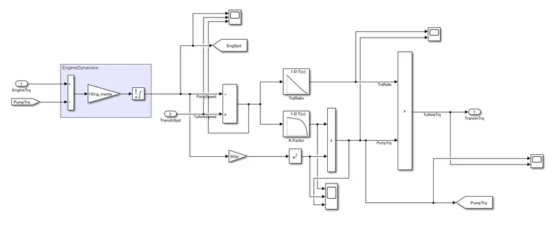
the gear selection from the transmission control is multiplied bu eng_trq and effeciency and dynamics of engine is done here.
DIFFERENTIAL MODEL:
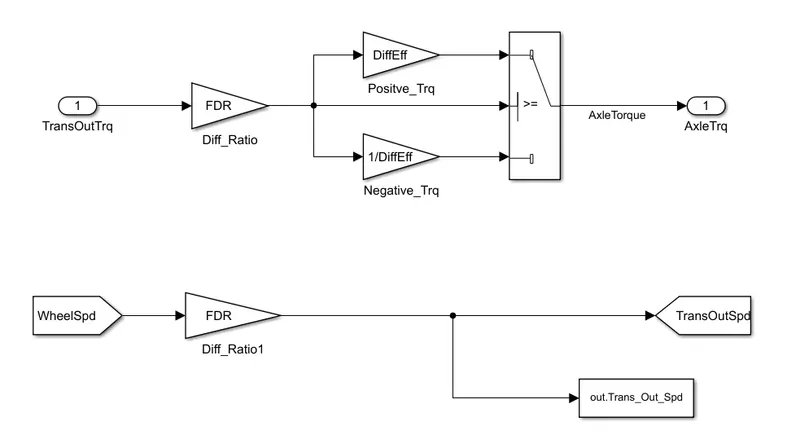
it provides the power output to the wheels according to their needs. the transmission is multiplied by differential ratio and efficiency.
WHEEL MODEL:
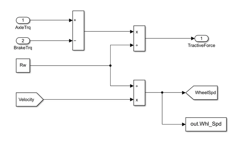
the brake torque is subtracted from the axle torque and divided by rolling radius to find tractive force of the system.
the speed of the wheels is found from the vehicle velocity.
VEHICLE DYNAMICS:
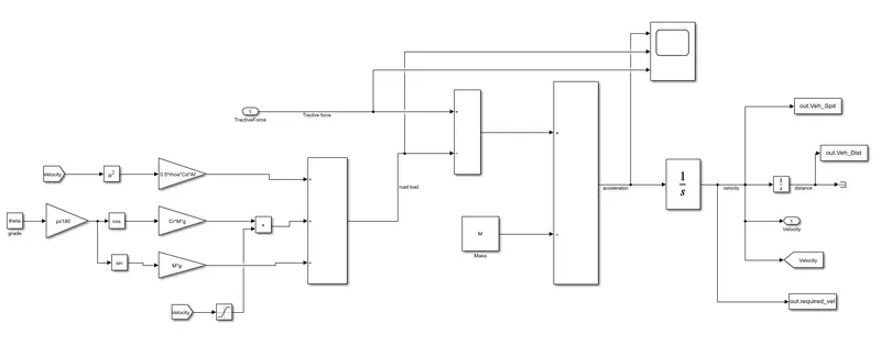
the dynamics and the road load of the vehicle is stated here.
tractive force and road load is used to find the velocity of the vehicle.

this equation forms the base for the vehicle dynamics block.
rhoa = density of air.
Af = frontal area
Cr = rolling coefficient.
M = mass
g = gravity.
theta = slope.
SIMULATION RESULTS:
FOR UDDC
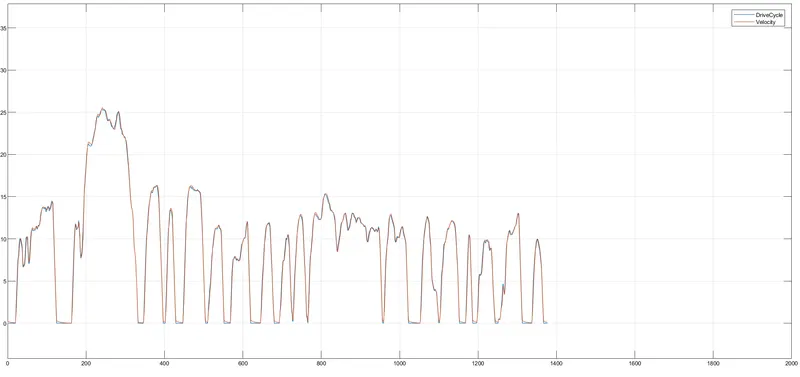
DRIVE CYCLE AND VELOCITY:
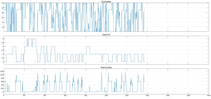
ENGINE TORQUE, GEAR COMMAND, BRAKE TORQUE(CONTROL UNIT):
FUEL RATE, FUEL CONSUMPTION:
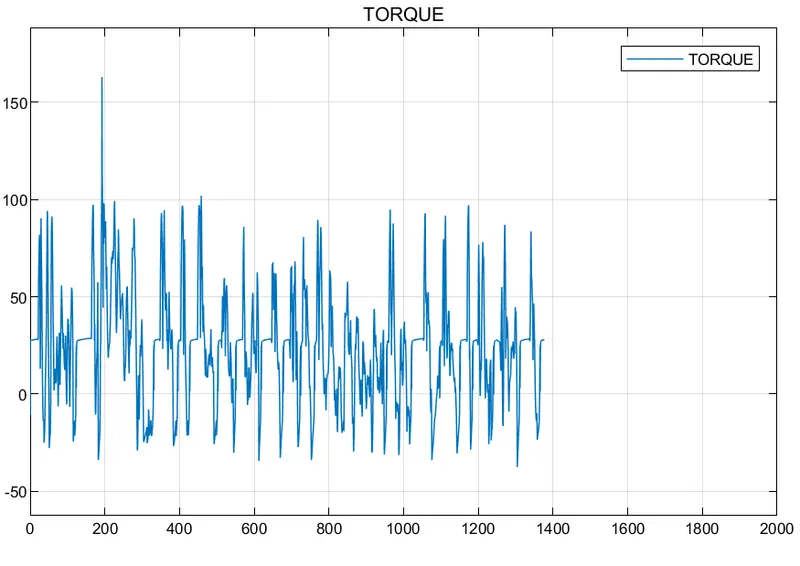
ENGINE TORQUE:
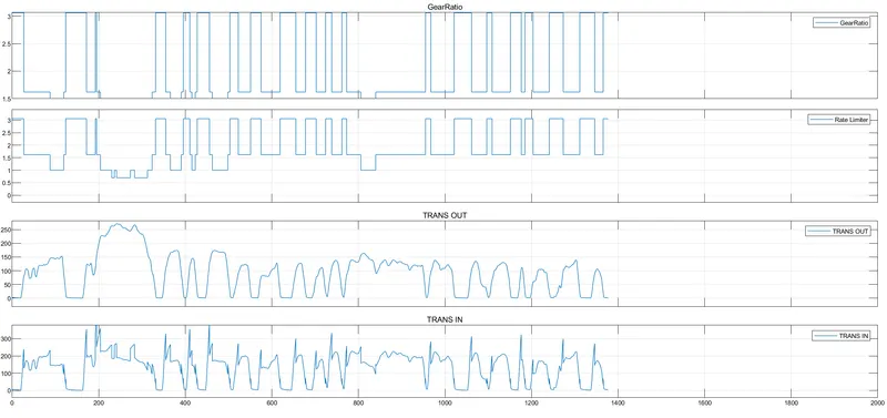
GEAR RATIO, TRANSMISSION INPUT, TRANS OUTPUT:
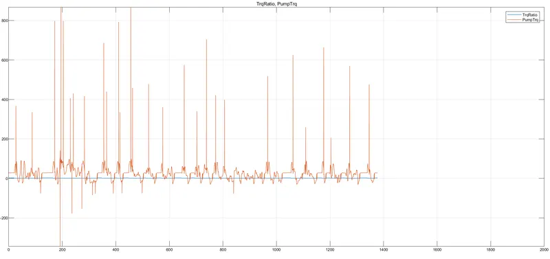
TORQUE RATIO AND PUMP TORQUE(TORQUE CONVERTER):
PUMP SPEED, TURBINE SPEED:
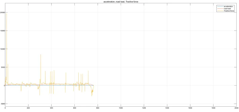
LOAD, TRACTIVE FORCE, ACCELERATION:
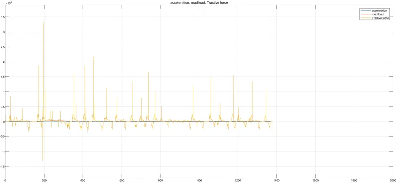
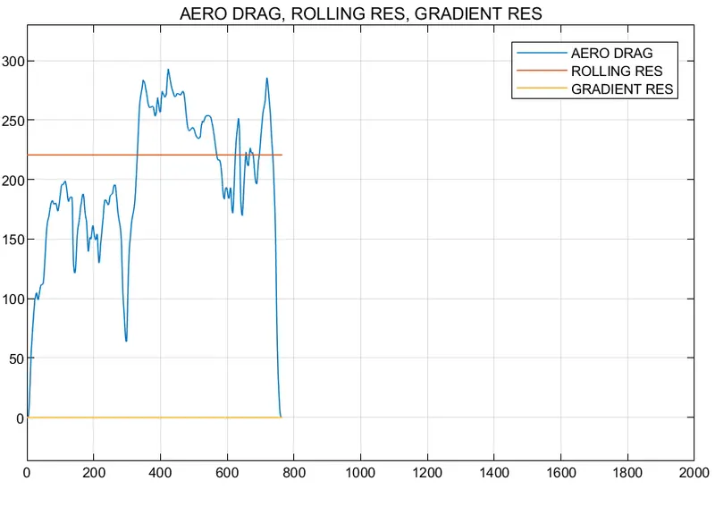
ROAD LOADS:
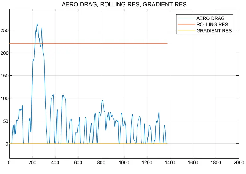
FOR HWFET CYCLE:
DRIVE CYCLE AND ACTUAL VELOCITY:
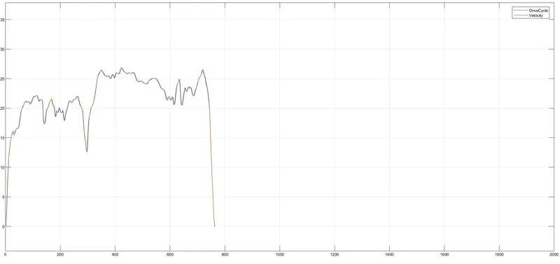
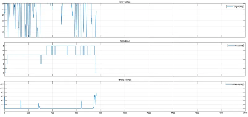
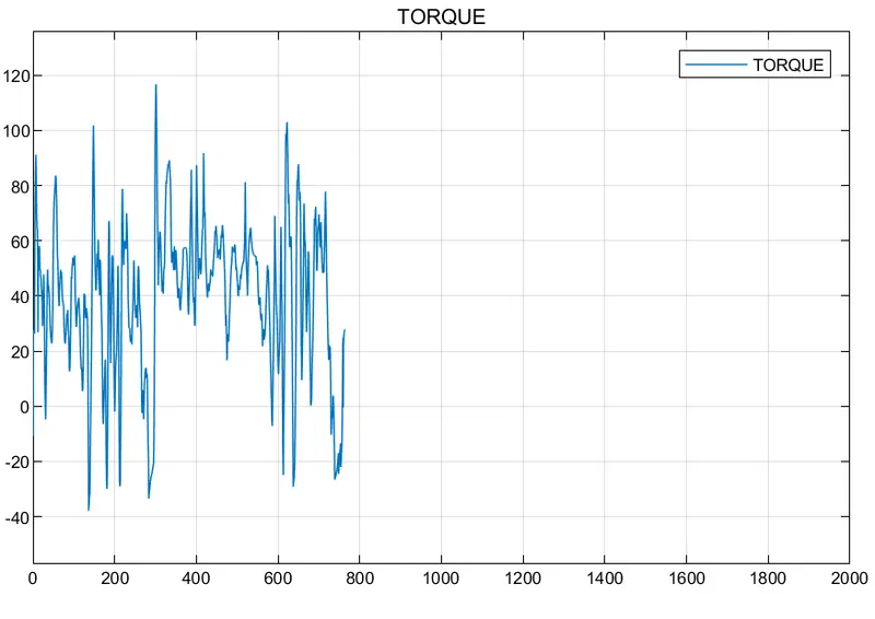
ENGINE TORQUE,BRAKE TOR, GEAR:
FUEL RATE AND FUEL CONSUMPTION:
ENGINE TORQUE:
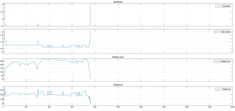
GEAR RATIO, TRANS IN AND OUTPUT SPEED:
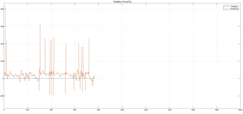
TORQUE RATIO AND PUMP TORQUE:
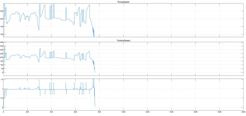
PUMP SPEED,TURBINE SPEED:
ROAD LOADS:
TRAC FORCE, ROAD LOAD, ACCELERATION:
................................................................................................................................................................................................................................................................................................................................................................
POST PROCESSING OF THE DATA:
CODE FOR PROCESSING:
%%%%%%%%%%%%%%%%%%%%%%%%%%%%%%%%%%%%%%%%%%%%%%%%%%%%%%%%%%%%%%%%%%%%%
%% Skill-Lync -> Hybrid Drives Development
% Project 1 - Conventional Vehicle Model
% By - SIKKANDAR FAIZ

% Description:
% The following file is to used with the Initialization file and Simulink
% results for post-processing of the data.
% The file is incomplete, has some examples of how the data is imported
% into a readable format, data analysis and plotting examples.
% Based on the project task, use commands in a similar format as given
% below, to analyse the data and generate required plots.
% You can change variable names if desired

%% Post-Processing File
%  File for post-processing the Conventional vehicle simulation model data

%% Renaming variables
Time = out.tout;
Acc_Pdl = out.Acc_Pdl;          % Accelerator pedal [%]
Brk_Pdl = out.Brk_Pdl;          % Brake pedal [%]
Gear_Cmd = out.Gear_Cmd;        % Transmission gear
Trans_In_Spd = out.Trans_In_Spd*30/pi;  % Transmission input speed [rpm]
Trans_Out_Spd = out.Trans_Out_Spd*30/pi;% Transmission output speed [rpm]
Eng_Trq = out.Eng_Trq;          % Engine brake torque [Nm]
Eng_Spd = out.Eng_Spd*30/pi;    % Engine speed [rpm]
Eng_Fuel_Consump = out.Eng_Fuel_Consumption;    % Engine fuel consumption [g]
Veh_Dist = out.Veh_Dist/1000;   % Distance traveled by vehicle [km]
Veh_Spd = out.Veh_Spd*18/5;     % Vehicle speed [kmph]
Whl_Spd = out.Whl_Spd*30/pi;
Required_speed = out.required_vel*18/5;
Eng_Fuel_Rate = out.Eng_Fuel_Rate;


%% Data Analysis
Eng_Pwr = Eng_Spd.*pi/30.*Eng_Trq/1000;   % Engine brake power [kW]
rho_petrol = 0.7197;                    % Density of petrol [kg/L]
kmpl = Veh_Dist(end)/(Eng_Fuel_Consump(end)/1000/rho_petrol);    % Fuel economy [kmpl]

%showing the fuel economy of the vehicle:
fprintf('Fuel Economy = %2.1fkmplnn',kmpl);

%% Plotting vehicle characteristics time trace

%plotting for transmission input, transmission output and wheel speed
figure(1)
hold on
grid on
plot(Time,Trans_In_Spd,'LineWidth',2,'color','r');
plot(Time,Trans_Out_Spd,'LineWidth',2,'color','b');
plot(Time,Whl_Spd,'LineWidth',2,'color','g');
xlabel('Time(s)')
ylabel('speed(rpm)')
xlim([0,Time(end)]);
legend('trans input','trans output','wheel speed');

%plotting for engine torque, engine power, fuel rate, fuel consumption.
%we are to make 4 plots in same figure
figure(2)
subplot(4,1,1)
hold on
grid on
plot(Time,Eng_Trq,'linewidth',2,'color','r');
ylabel('torque(NM)')
xlim([0,Time(end)])

subplot(4,1,2)
hold on
grid on
plot(Time,Eng_Pwr,'linewidth',2,'color','b');
ylabel('Power(KW)')
xlim([0,Time(end)])

subplot(4,1,3)
hold on
grid on
plot(Time,Eng_Fuel_Rate,'linewidth',2,'color','g');
xlabel('Time(s)')
ylabel('Engine fuel rate')
xlim([0,Time(end)])

subplot(4,1,4)
hold on
grid on
plot(Time,Eng_Fuel_Consump,'LineWidth',2,'Color','k')
xlabel('Time(s)')
ylabel('Engine fuel consumption')
xlim([0,Time(end)])

%plotting acceleration, brake pedal, gear command, vehicle required and
%actual speed, vehicle distance.
%we are to make 4 plots in same figure
figure(3)
subplot(4,1,1)
hold on
grid on
plot(Time,Acc_Pdl,'LineWidth',2,'Color','r')
plot(Time,Brk_Pdl,'LineWidth',2,'Color','b')
ylabel('pedal')
xlim([0,Time(end)]);
legend('acceleration','brake')

subplot(4,1,2)
hold on
grid on
plot(Time,Gear_Cmd,'LineWidth',2,'Color','g')
xlabel('Time(s)')
ylabel('Gear')
xlim([0,Time(end)]);

subplot(4,1,3)
hold on
grid on
plot(Time,Veh_Spd,'LineWidth',2,'Color','k');
plot(Time,Required_speed,'LineWidth',2,'Color','c')
ylabel('speed(kmph)')
xlim([0,Time(end)])
legend('actual speed','required speed')

subplot(4,1,4)
hold on
grid on
plot(Time,Veh_Dist,'LineWidth',2,'Color','m')
xlabel('Time(s)')
ylabel('distance(km)')
xlim([0,Time(end)])


%plotting drive cycle
figure(4)
hold on
grid on
plot(cyc_time,cyc_vel,'LineWidth',2,'Color','r')
xlabel('Time(s)')
ylabel('distance(km)')
title('drive cycle')

%final code result
Average_speed = sum(Veh_Spd)/length(Veh_Spd);
Max_speed = maxk(Veh_Spd,1);
table(Average_speed,Max_speed,kmpl,'variablenames',{'average speed[kmph]','maximum speed[kmph]','fuel economy[kmph]'})

%% Plotting engine operating points on engine fuel map
figure('Name','Engine Operating Points');
hold on
grid on
title('Engine Operating Points','fontsize',12);
p1=plot(Eng_map_spd*30/pi,Eng_max_trq,'linewidth',2,'color','r');
p2=line([Eng_map_spd(end)*30/pi Eng_map_spd(end)*30/pi],[0 Eng_max_trq(end)]);
set(p2,'linewidth',1,'linestyle','--','color','k');
p3=line([Eng_map_spd(1)*30/pi Eng_map_spd(1)*30/pi],[0 Eng_max_trq(1)]);
set(p3,'linewidth',1,'linestyle','--','color','k');
[c,h] = contour(Eng_map_spd'*30/pi,Eng_map_trq,Eng_fuel_map');
clabel(c,h);
xlabel('Engine Speed [rpm]');
ylabel('Engine Torque [Nm]');
title('Engine Fuel Consumption Map [g/s]');
% p4 = plot(Eng_Spd,Eng_Trq,'.','color','k');
legend([p1 p3],{'Max Curve','Operating Points'});
axis([Eng_map_spd(1)*30/pi Eng_map_spd(end)*30/pi 0 Eng_map_trq(end)]);
POST PROCESSING RESULT FOR UDDC CYCLE:
FUEL ECONOMY AND AVER AND MAX SPEED:
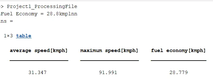
fuel economy is less than the HWFET cycle.
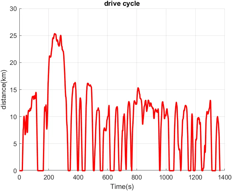
UDDC DRIVE CYCLE:
TRANSSMISSION INPUT, TRANS OUTPUT, WHEEL SPEED:
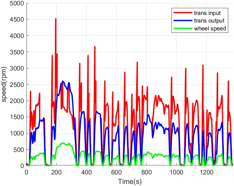
wheel speed and transmission output vary according to gear and diff ratio.
ENGINE TORQUE, ENG POWER, FUEL RATE, FUEL CONSUMPTION:
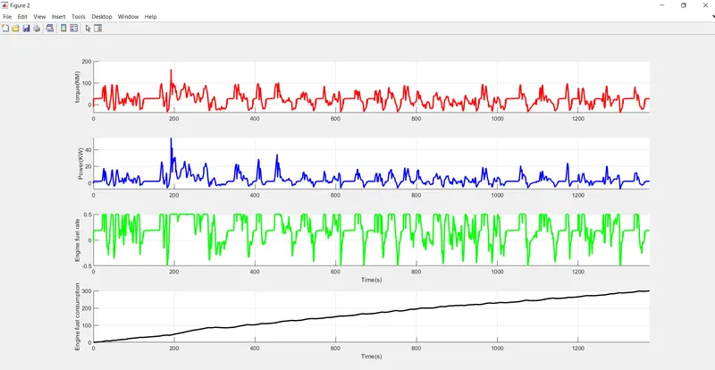
the torque requirements is different for drive cycles.
ACCELERATOR, BRAKE PEDAL,GEAR, REQUIRED SPEED,DISTANCE:
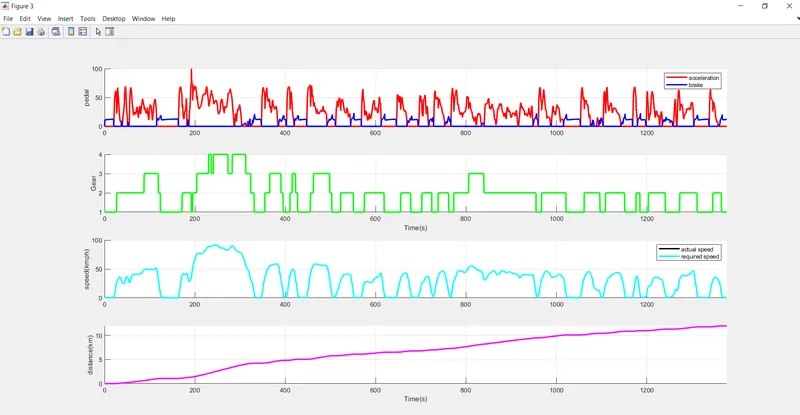
acceleration and brake are used more the cycle is not smooth.gear hould be shifted frequently.
ENGINE OPERATING POINTS ON ENGINE FUEL MAP:
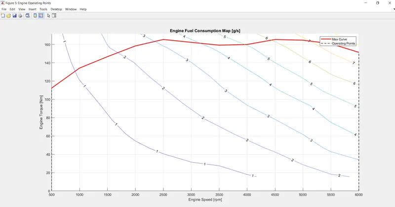 operating points are under max torque curve.
................................................................................................................................................................................................................................................................................................................................................................
POST PROCESSING RESULT FOR HWFET CYCLE:
FUEL ECONOMY AND AVER AND MAX SPEED:
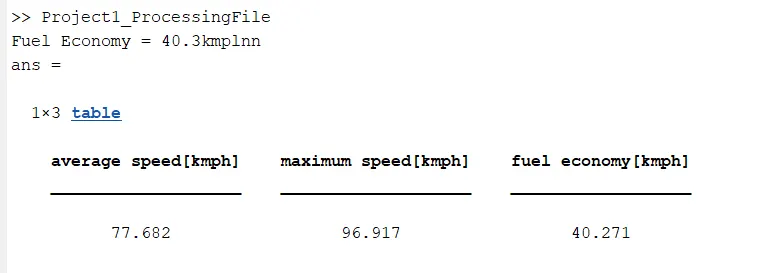
economy is high than uddc.
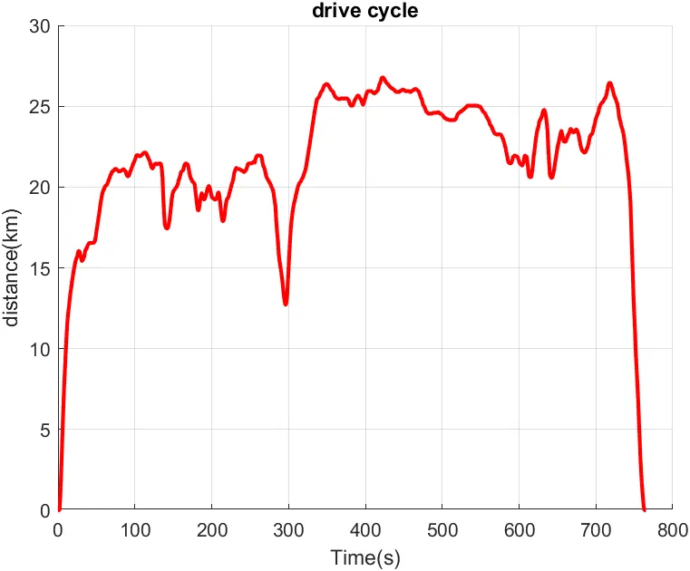
HWFET DRIVE CYCLE:
TRANSSMISSION INPUT, TRANS OUTPUT, WHEEL SPEED:
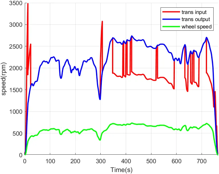
wheel speed and transmission output vary according to gear and diff ratio.
ENGINE TORQUE, ENG POWER, FUEL RATE, FUEL CONSUMPTION:
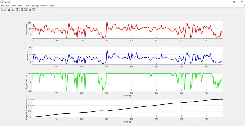
the torque requirements is different for drive cycles. and the fuel requirements too.
ACCELERATOR, BRAKE PEDAL,GEAR, REQUIRED SPEED,DISTANCE:
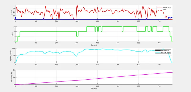
brake requirement is not much needed in highway and the gear shifts are not too frequent too, this helps in smooth drive cycle.
ENGINE OPERATING POINTS ON ENGINE FUEL MAP:
conclusion:
the given data is well studied and the asked conditions:
a. Tabulate the fuel economy numbers (kmpl) for UDDS and HWFET cycle. This forms the baseline numbers for comparing with the future hybrid version.
b. Plot the time trace for engine, transmission input, transmission output and wheel speed on one plot.
c. Plot engine torque, engine power, fuel rate and fuel consumption using subplots.
d. Plot accelerator and brake pedal, gear command, vehicle desired and actual speed, vehicle distance using subplots.
e. Plot the engine operating points on the engine fuel map.
f. Write down appropriate brief comments on each of these plots, describing the vehicle behavior throughout the drive cycle.
g. Generate the plots for both drive cycles
are satisfied.