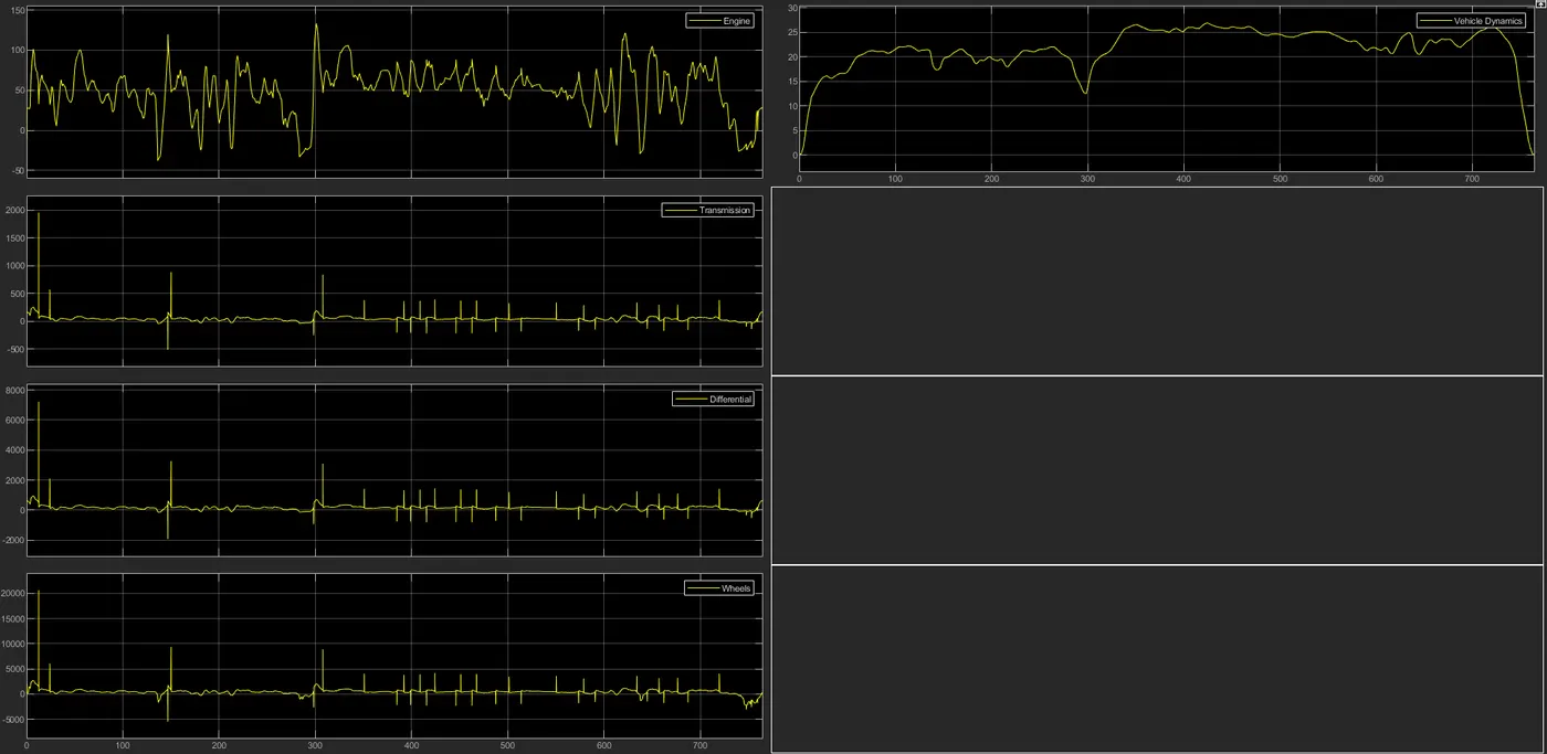
Project 1
UDDS cycle result:
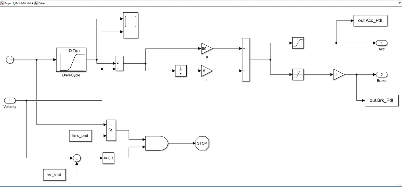
For driver model - it is a basic PI controller that generates accelerator and brake pedal outputs to match the desired and actual vehicle speeds.
cycle velocity and cycle time are fed to the lookup table. the output is then added and integrated in the PI controller which is then saturated and fed to
the workspace. when time and velocity ends, the simulation stops.
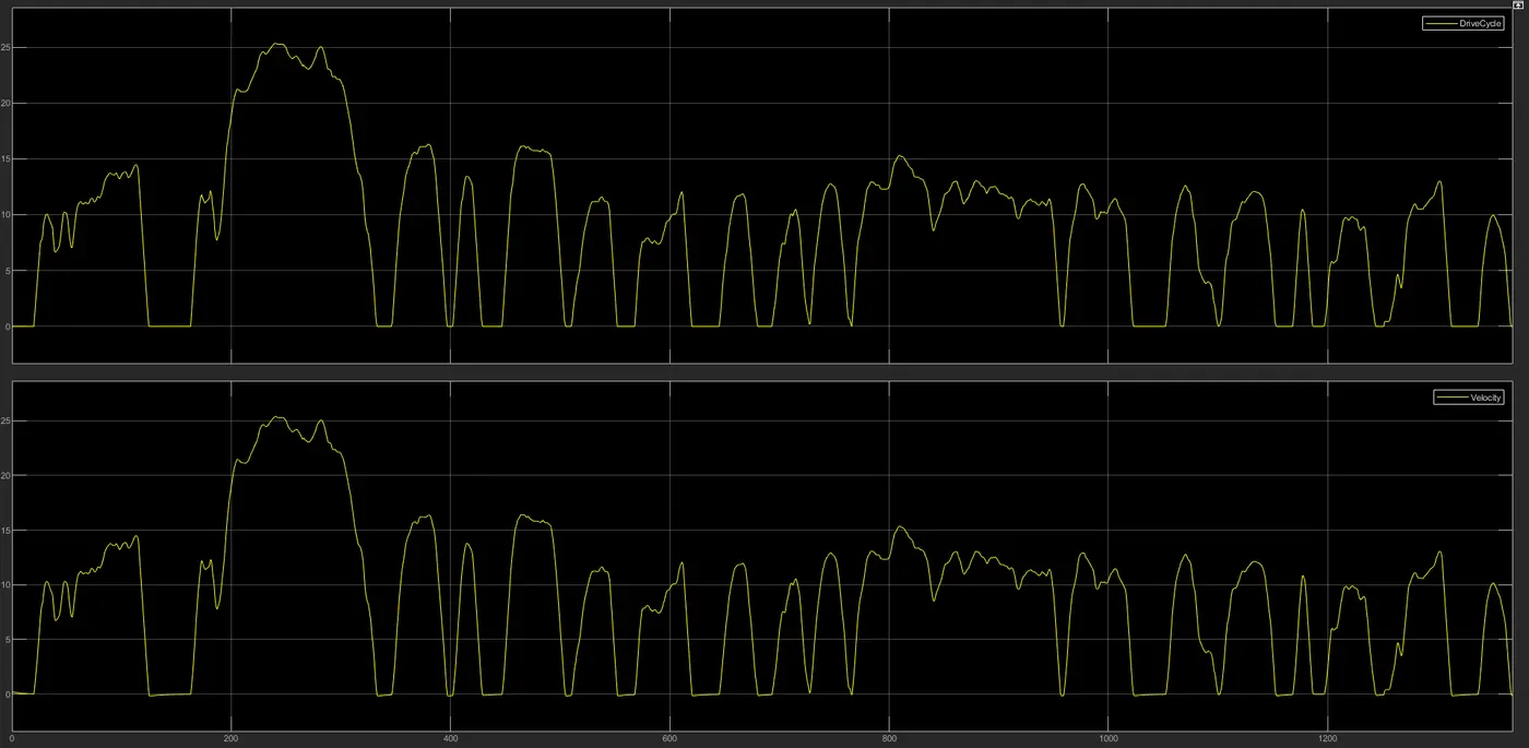
The velocity and drive cycle graph is shown above. They should be similar flowing graphs which they are after output.
the acceleration and brake inputs are fed to the controller unit. it is the brains of the vehicle. basedon driver inputs, it generates desired input engine torque, gear command and brake torque.
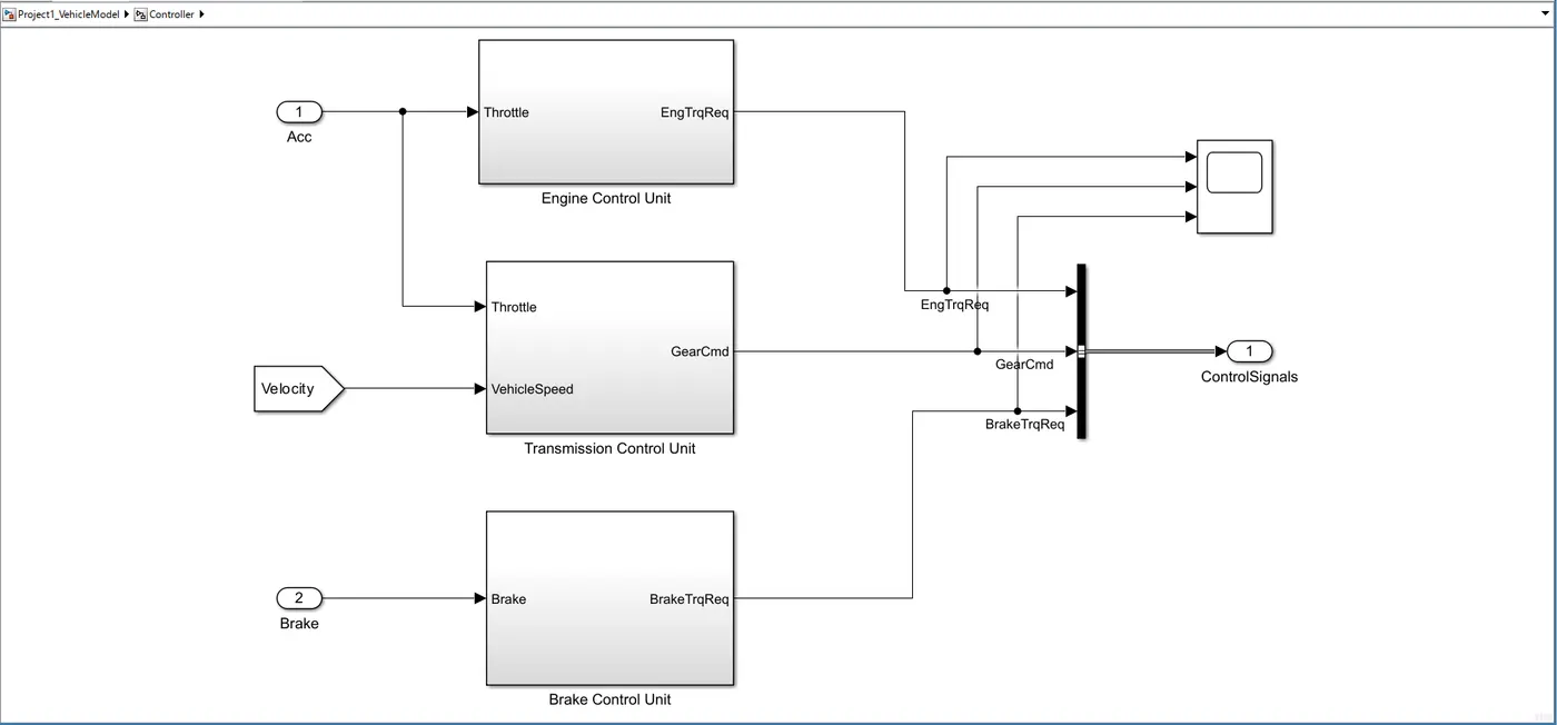
below is the output graph of controller unit:
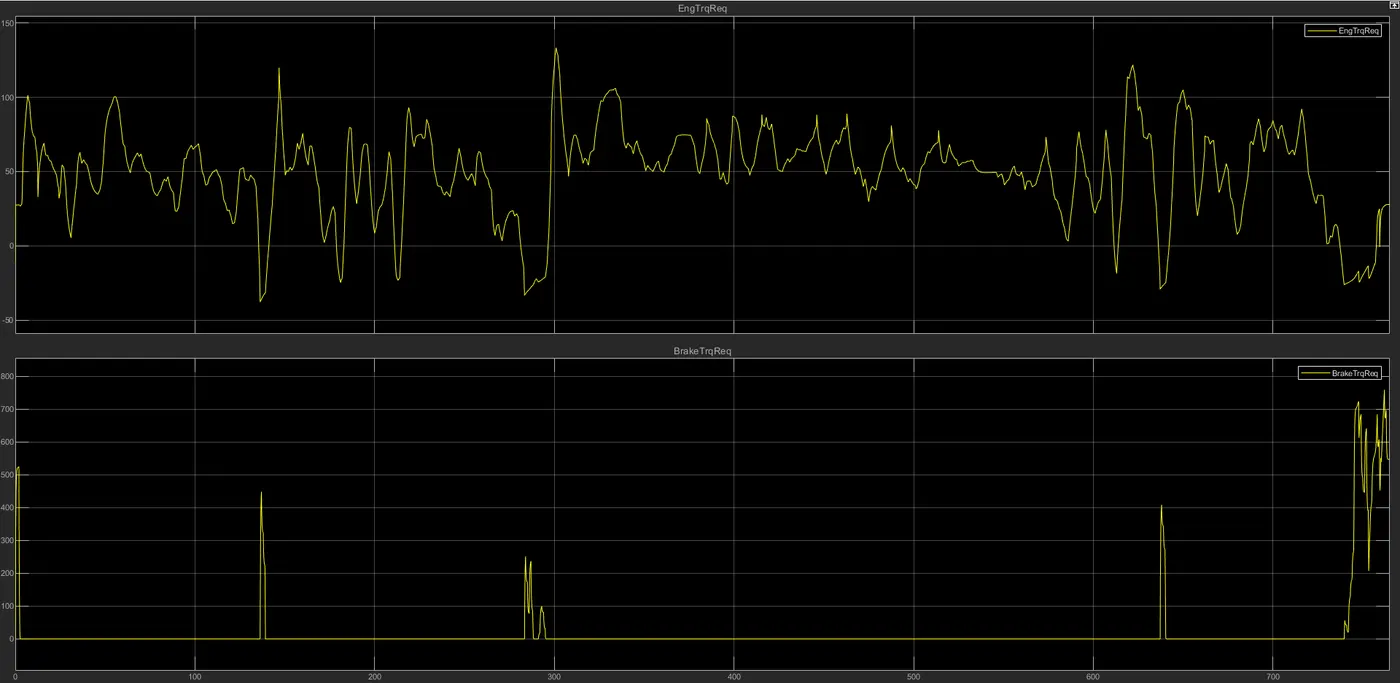
it shows the engine torque, brake torque and the gear the vehicle is riding in.
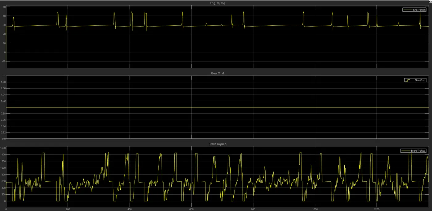
The graphs show the engine and the brake torque required with respect to time. The graphs vary according to the need on wheels and engine requirements. A better colored graph is plotted at the end of UDDS cycle for better understanding.
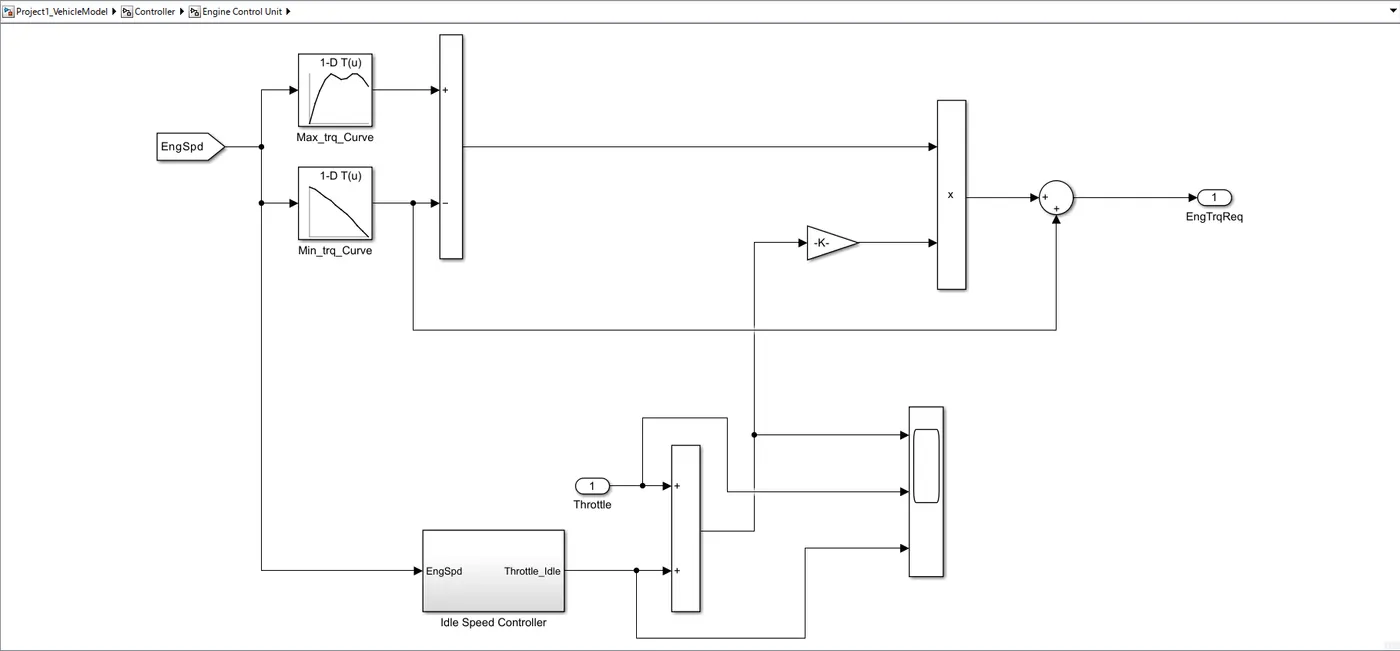
the engine control unit feeds the engine speed into max torque curve and minimum torque curve via lookup tables and then into the idle speed controller.
after the addition and subtraction blocks, the engine torque required is output.
below is the transmission contril unit:
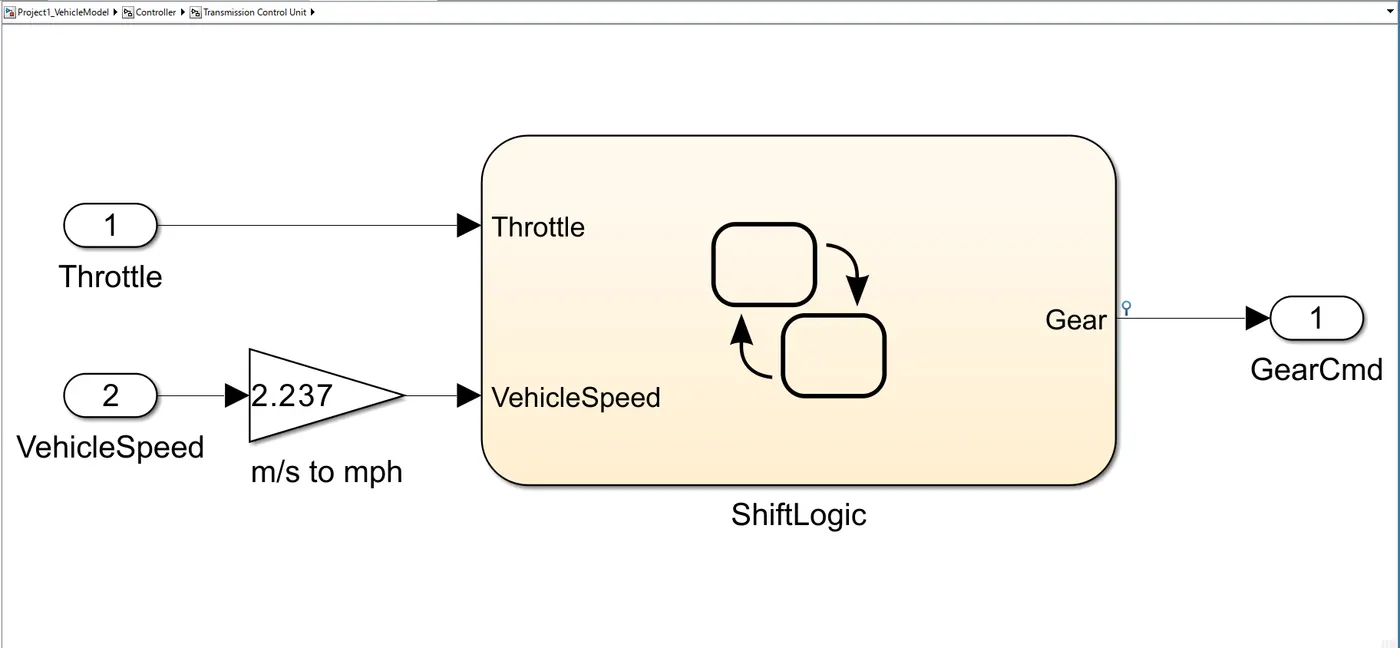
we give input to the gear change logic controller in mph. the gear change decision depends on the throttle and the vehicle speed.
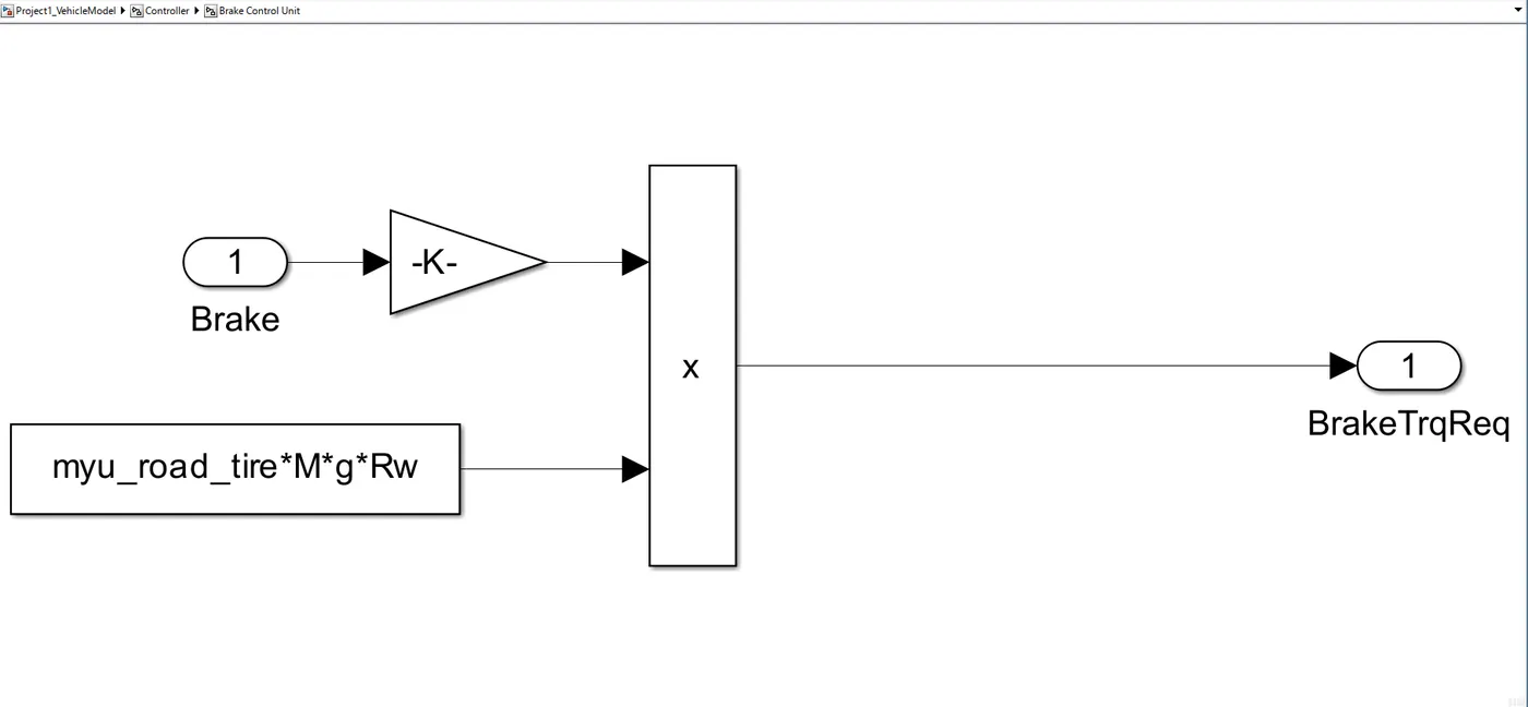
brake control unit calculates the brake torque required. then the control signals in the ofrm of engine torque required, brake torque required and gear command is then fed to the transmission unit in the form of control signals.
below is the engine powertrain image:
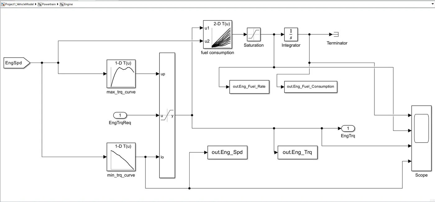
the engine control unit feeds the engine speed into max torque curve and minimum torque curve via lookup tables and then into the idle speed controller.
after the addition and subtraction blocks, the engine torque required is output. the graphs of engine powertrain block is below:
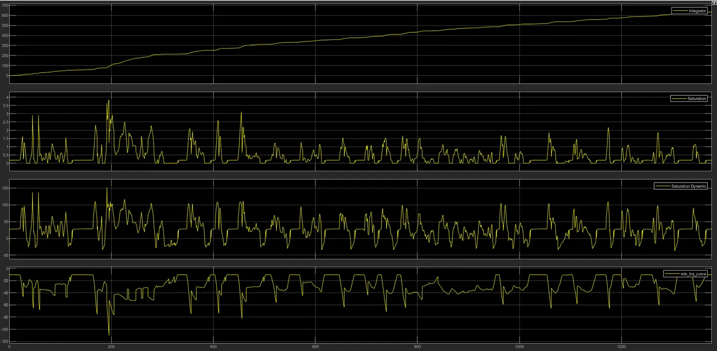
here, saturation is the engine fuel to air ratio graph. intrgrator is the engine fuel consumption graph. dynamic saturation is the engine speed graph. We need more fuel to air ratio when the power output required is more or increasing. When this ratio is satisfied, the engine output follows a similar trends.
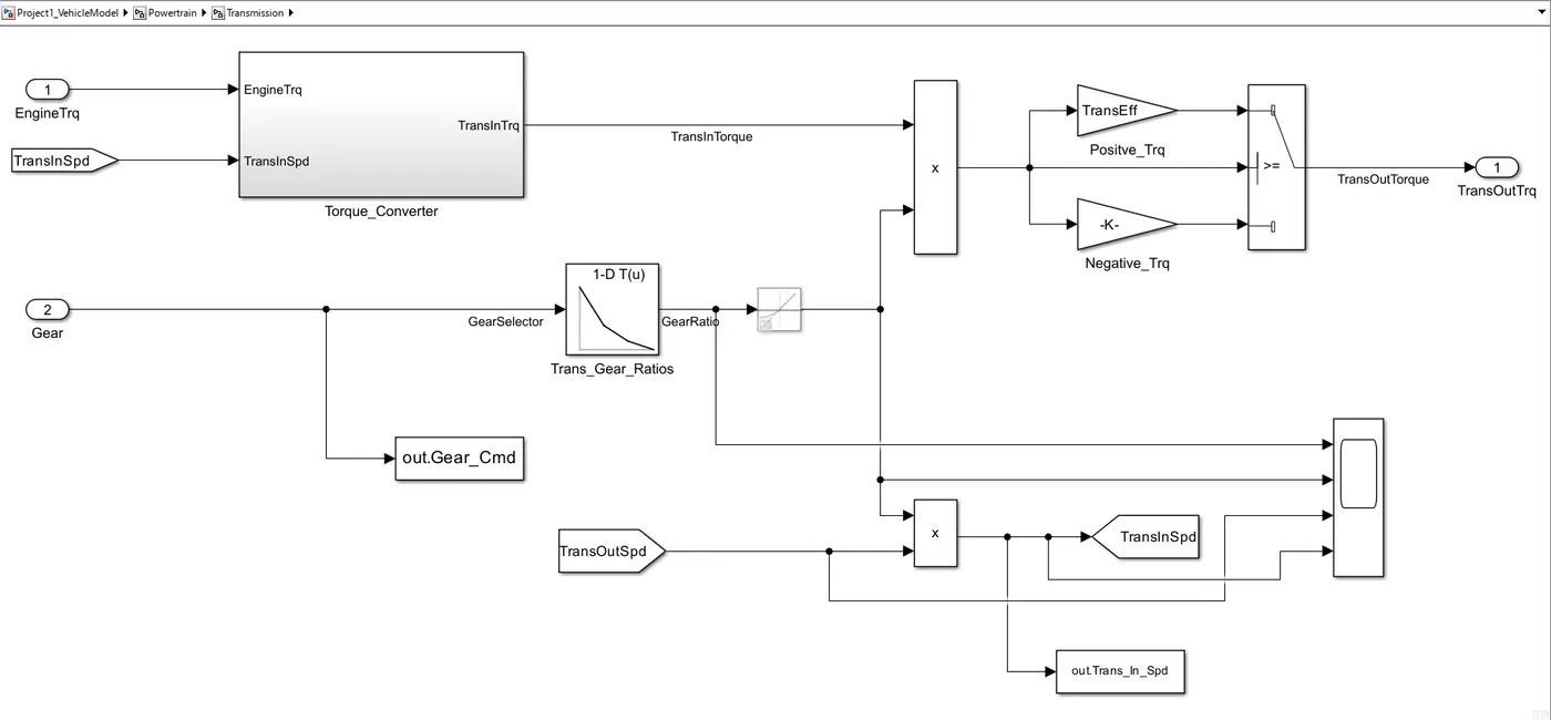
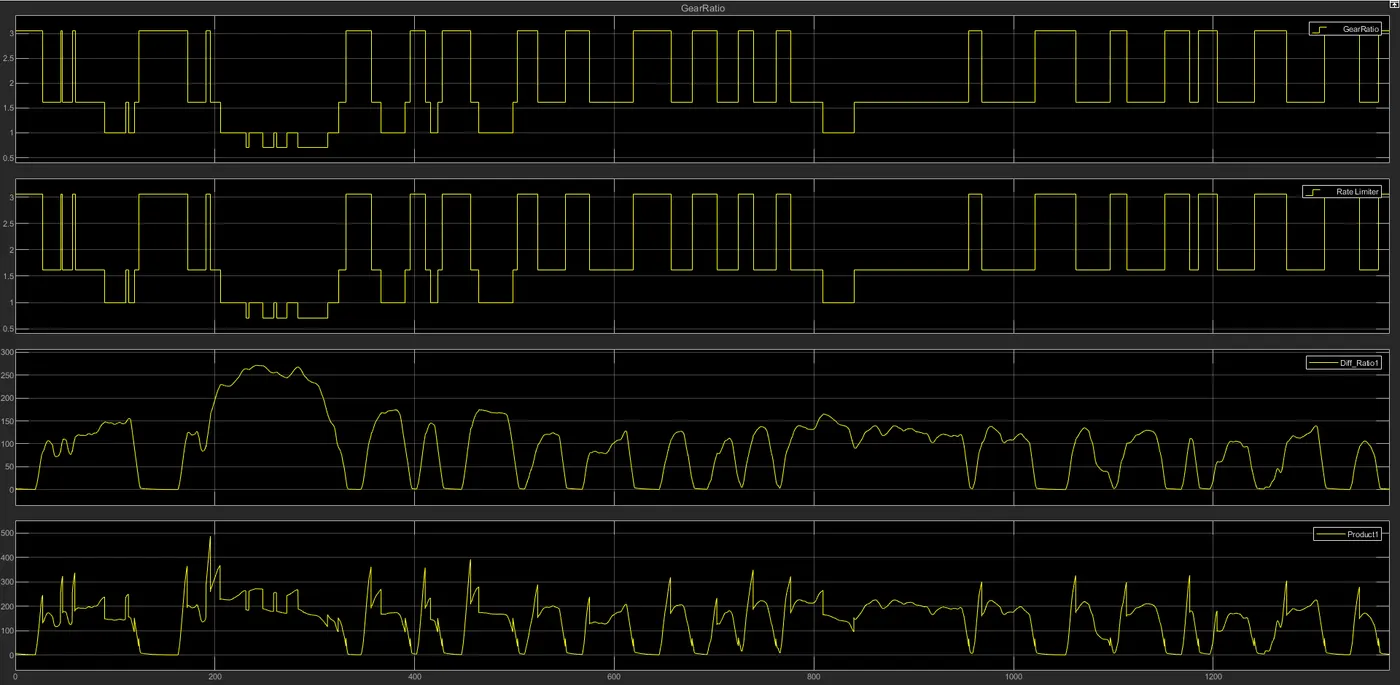
the gear ratio and rate limiter graphs are identical here. differential ratio and transitional speed are also output. in this model, we take engine torque, gear selector for transmission of gear ratio. the gear ratio is then multiplied by transmission input torque. This graph is seen in product1 and acts as transmission input speed. torque converter connects the engine to transmission.
below image is of differential:
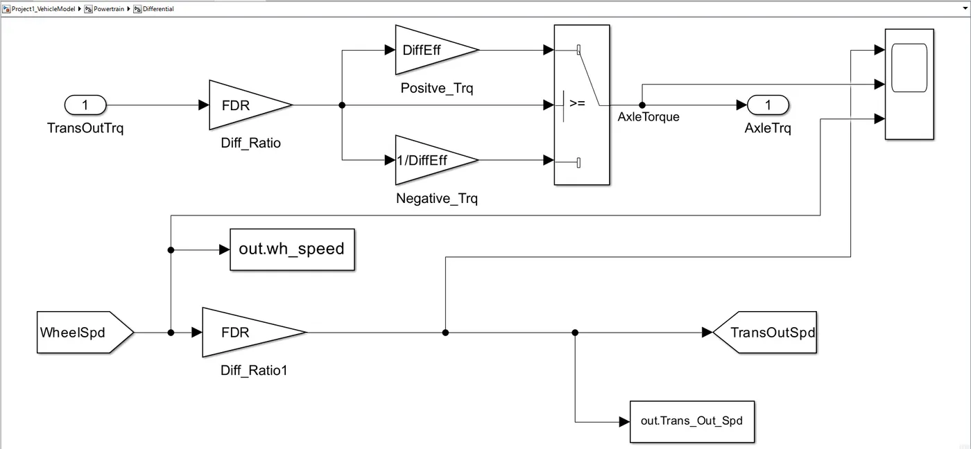
here, tranmisssion output otrque is fed through differential ratio finally to give axle torque via positive and negative torque filtering. wheel speed and transmission output speed also has a relation through this fixed differential ratio.
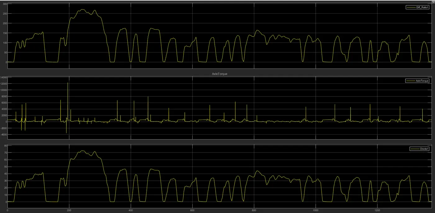
the above graphs shows transmission output speed, axle torque and wheel speed. the wheel and output speed have similar graphs. the axle torque acts whenever there is a change in the wheel speed.
in the wheels section, axle and brake torque are subtracted and divided by the wheel radius to get the tractive force and wheel speed is calculated dividing velocity by wheel radius. graphs are below:
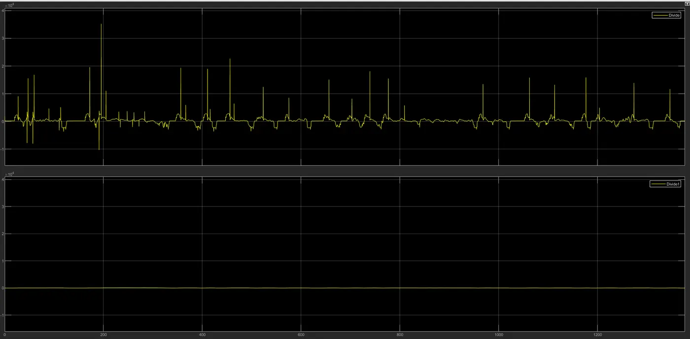
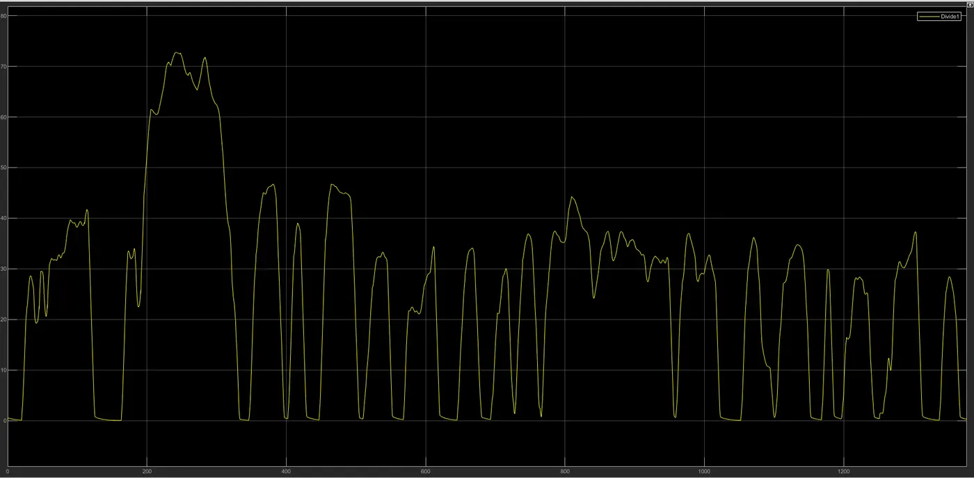
the wheel speed graph is shown more clearly in the below graph:
below is the vehicle dynamics image:
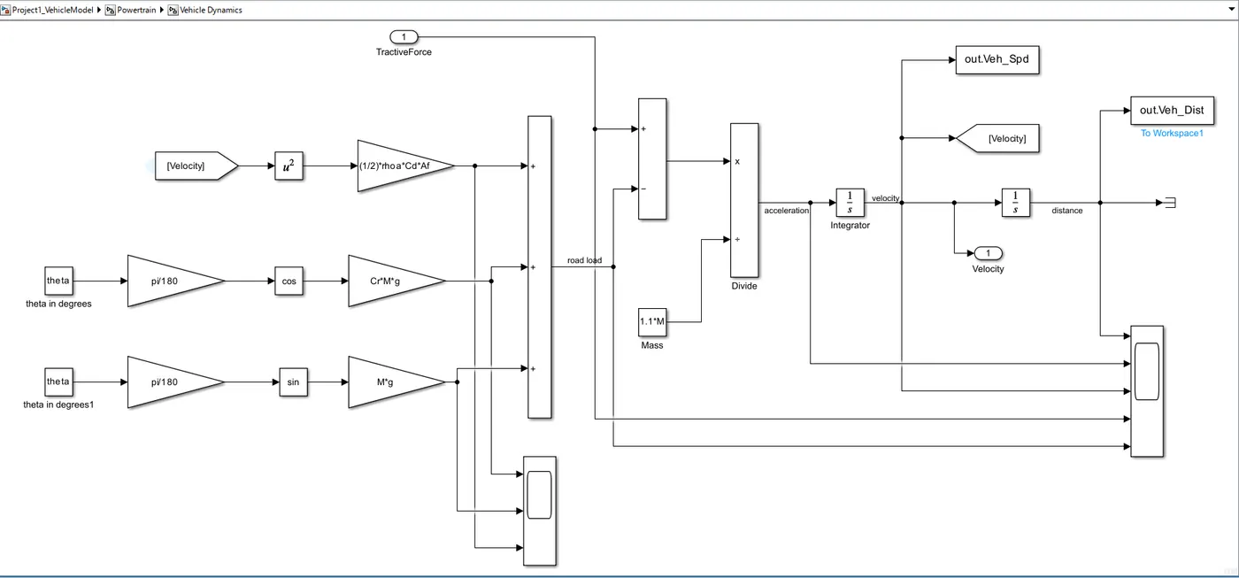
the dynamic equation for calculating road load is
MeqdVvehdt=ηtλtotRwTm-(12p⋅A⋅Cd⋅(Vveh+Vw∈d)2+Cr⋅M⋅g⋅cos(θ)+M⋅g⋅sin(θ))">MeqdVvehdt=ηtλtotRwTm−(12p⋅A⋅Cd⋅(Vveh+Vw∈d)2+Cr⋅M⋅g⋅cos(θ)+M⋅g⋅sin(θ))�������ℎ��=����������-(12�⋅�⋅��⋅(���ℎ+��∈�)2+��⋅�⋅�⋅cos(�)+�⋅�⋅sin(�))
where,
p = air density [kg/m^3]
A = Frontal area [m^2]
Cd = drag Coefficiend
Vveh = velocity of vehicle [m/s^2]
Vwind = velocity of wind [m/s^2]
Cr = rolling resistance coefficient
M = mass in [Kg]
g = gravity.
after the road load calculation from the above formula, it is subtracted from the tractive force and divided by the mass 1.1 times to count in the inertial mass factor.
this is the way we get acceleration. this is integrated to get velocity which is again integrated to get distance.
below is the graph of resistance forces:
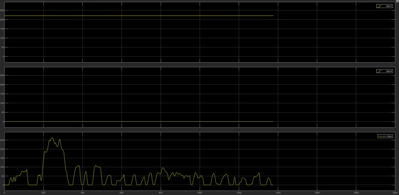
gain1 is constant rolling resistance force as theta is 0 degrees.
gain4 is grading force as theta is 0 degrees.
gain is the aerodynamic force which changes according to the velocity of vehicle.
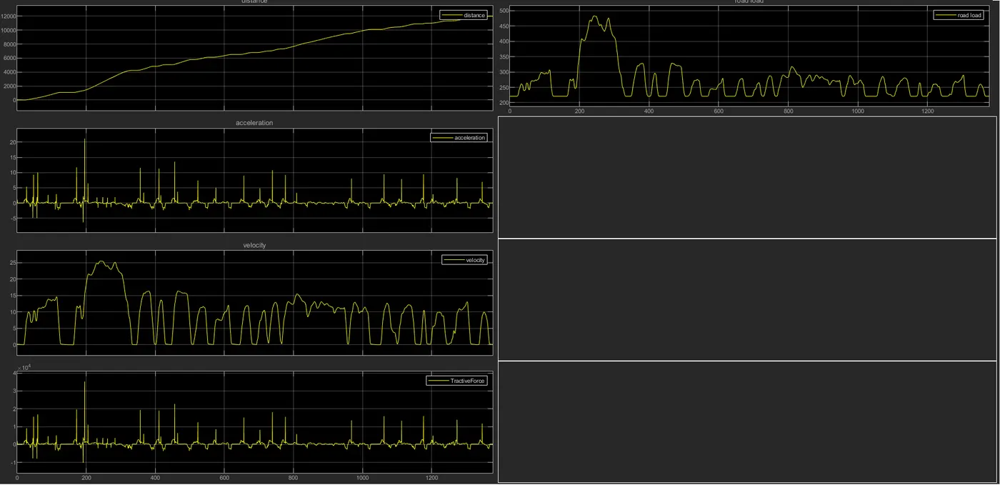
below is the distance, acc, vel, tractive force, road load graphs. Tractive force and acceleration have similar graphs. The distance goes on increasing irrespective of force or load conditions as the vehicle keeps on moving forward.
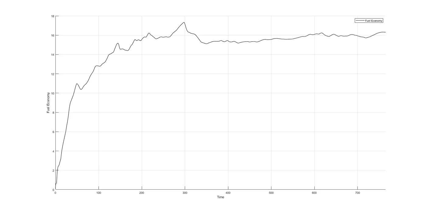
a. fuel economy numbers are as follows:
for UDDS:
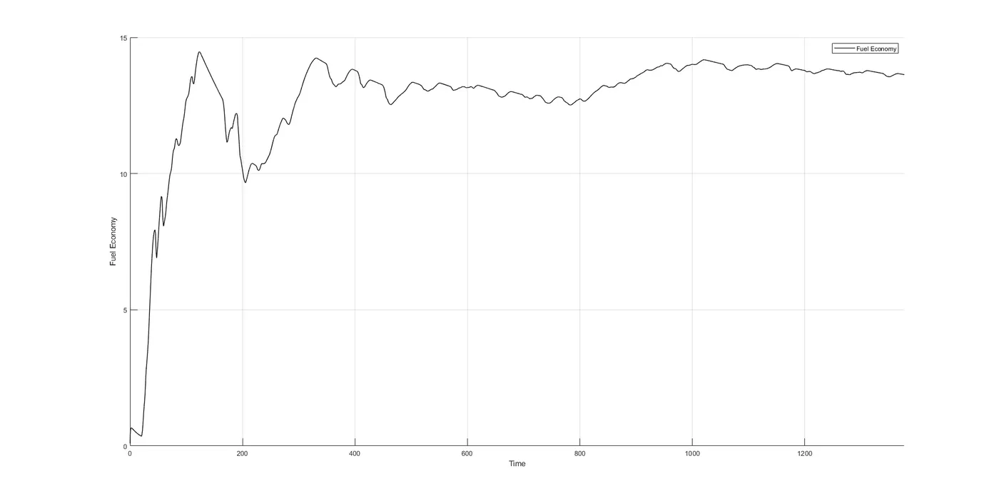
Fuel economy becomes almost constant after some amount of time. By graph it is 12.7455 kmpl (calculating mean of all values till end of time).
b.
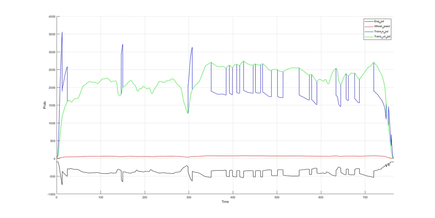
We can clearly see how different the transmission input and output speeds are. These are due to losses. Spikes seen in the former graphs are smoothened out in the latter graph. The engine speed and transmission input speed graphs have spikes at similar time instances. Finally the wheel speed is much less than both the transmission speeds.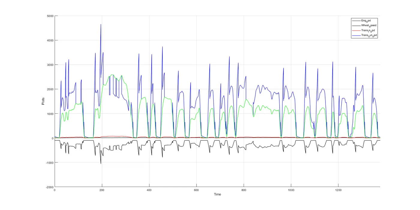
c.
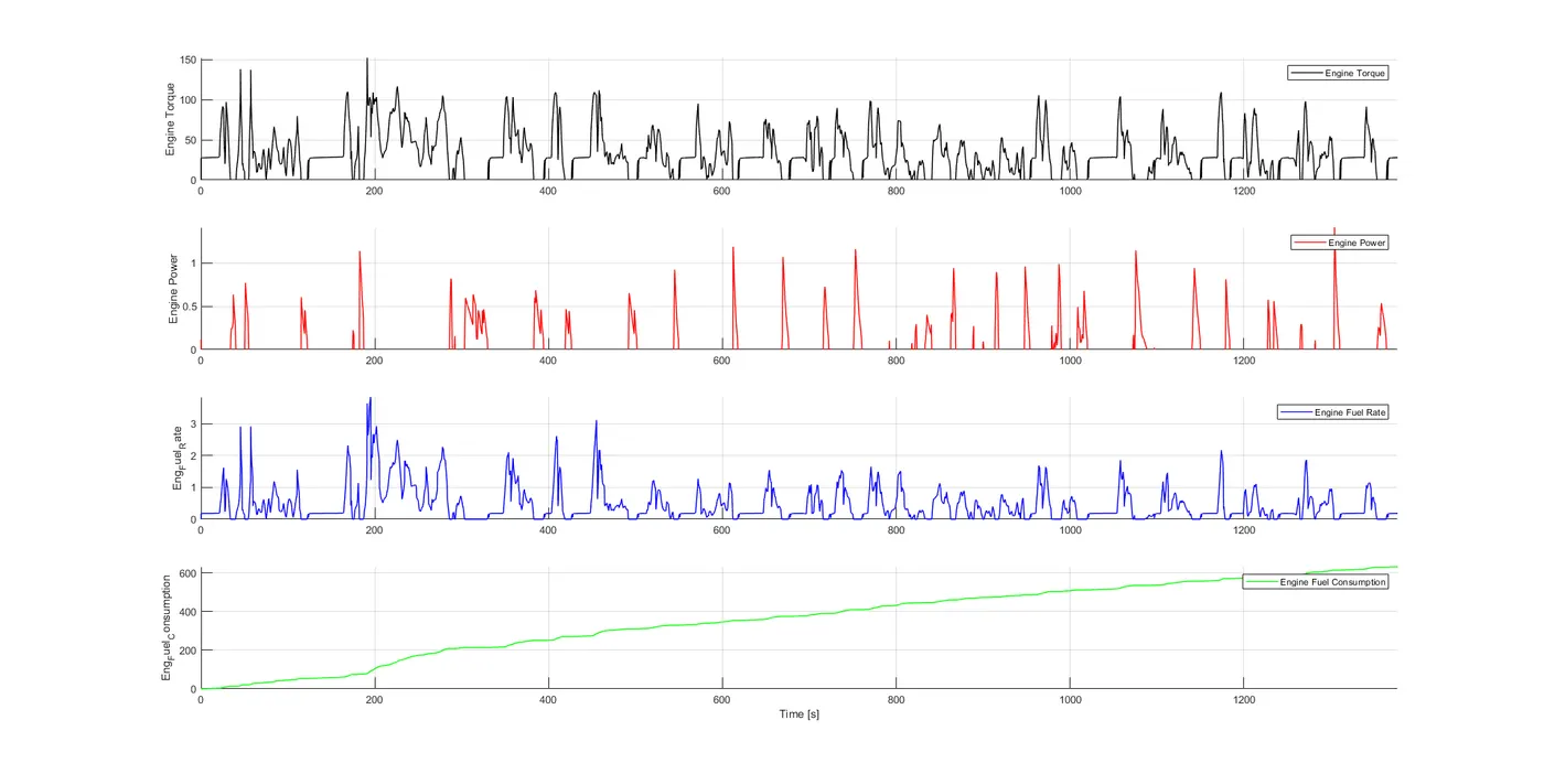
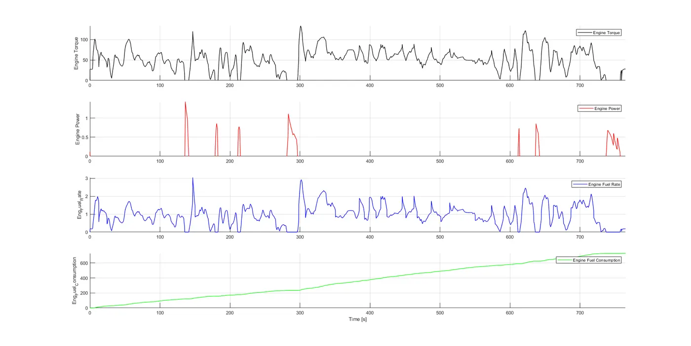
The engine fuel ratio demand goes hand in hand with the engine torque or the torque required at the wheels, which varies and depends solely on the input driver model. A rich fuel to air ratio is needed to satisfy the high torque and power demand of the engine. Subsequently, the fuel consumption always goes on increasing.
d.
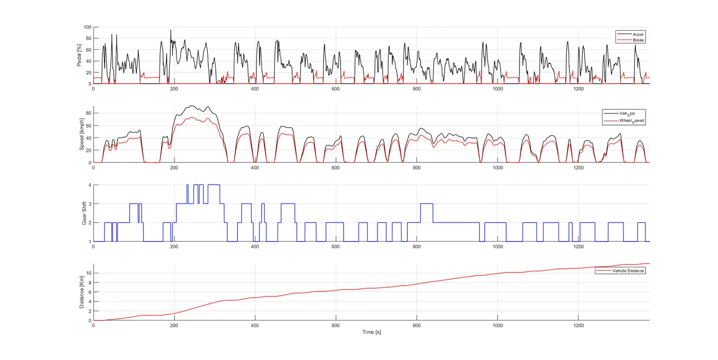
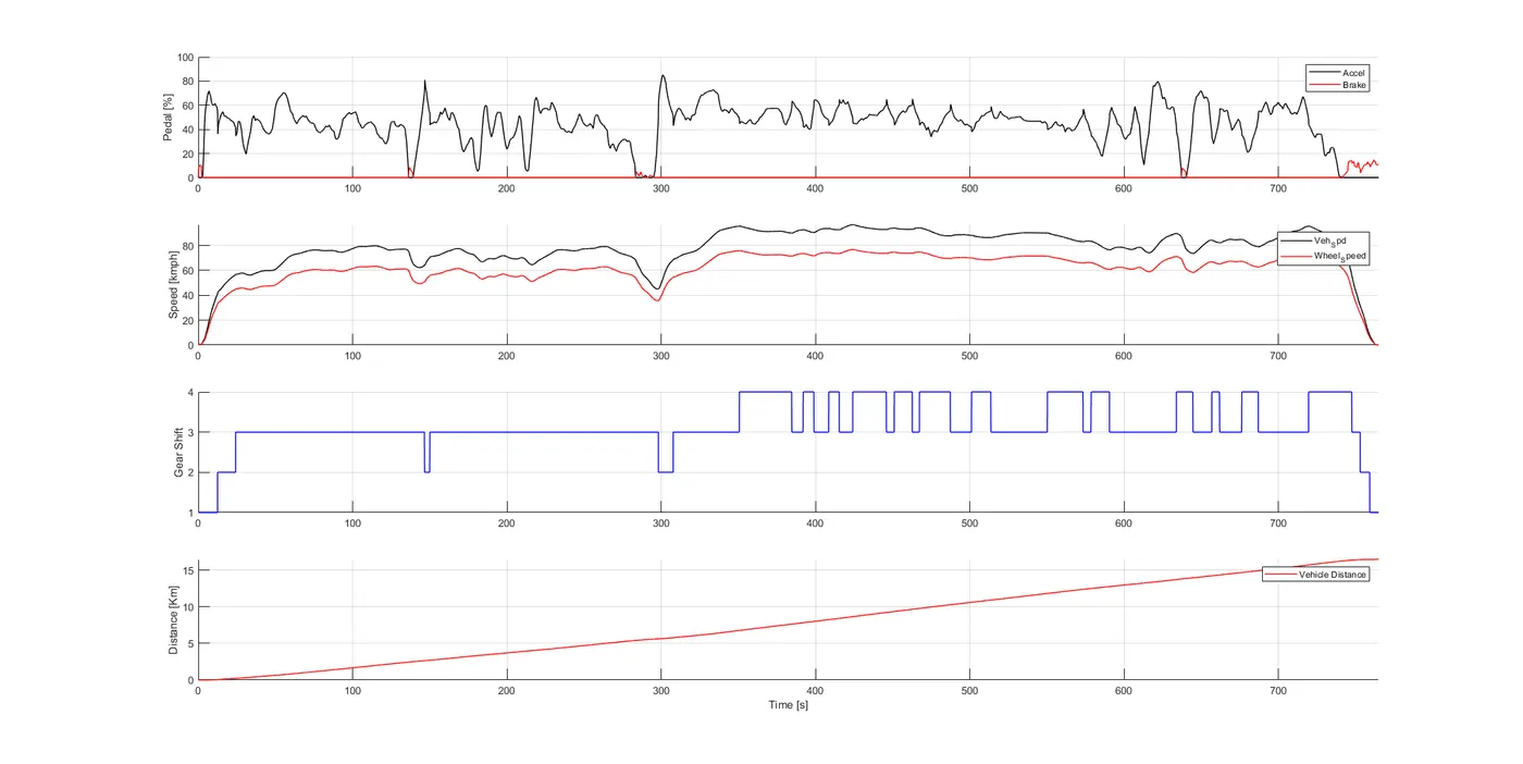
To satisfy the acceleration pedal input, change in gears is necessary. The vehicle desired and actual speed at the wheels is shown in the graphs. The difference signifies the loss in power due to default inefficiency. The vehicle distance increases as the vehicle propels forward.
e.
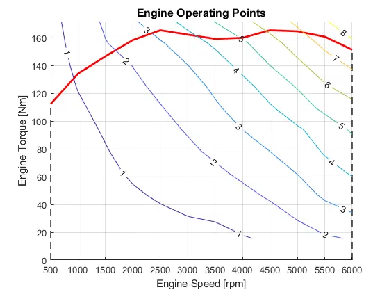
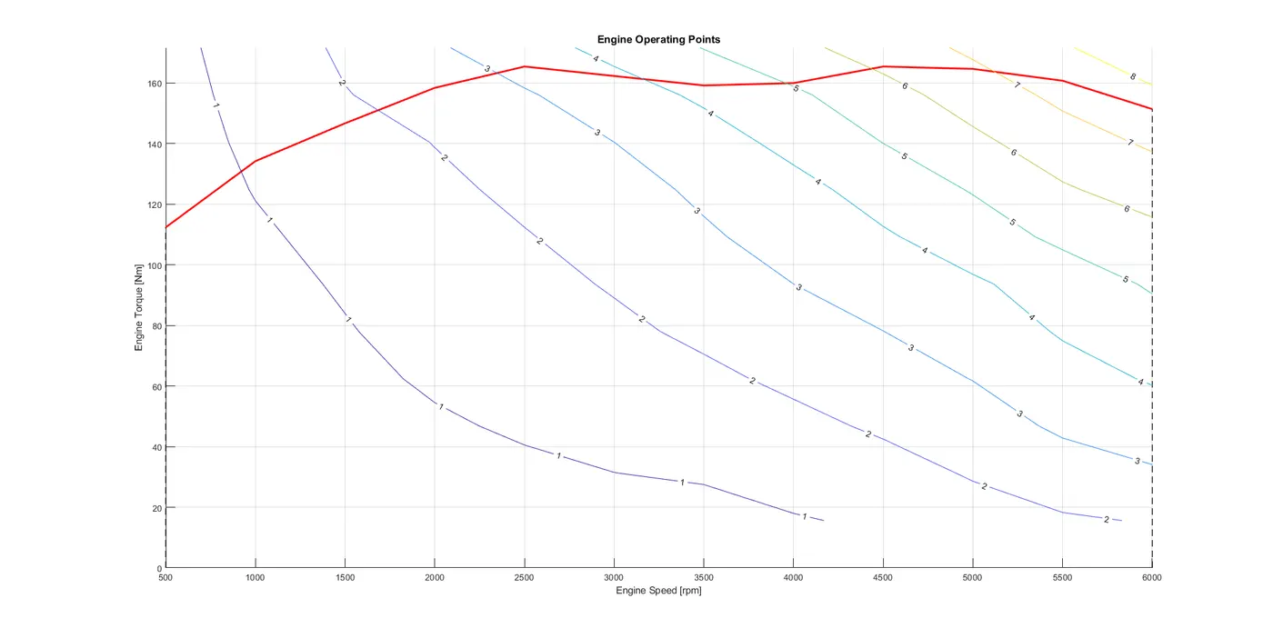
In the above image, the operating engine points are shown wrt. Engine speed and torque.
Results for HWFET cycle:
the driver model design in simulink remains the same. the graph for drive cycle and velocity is below:
change in <> is Drive_Cycle_Select = 2; % Drive cycle selection
where if Drive_Cycle_Select == 1
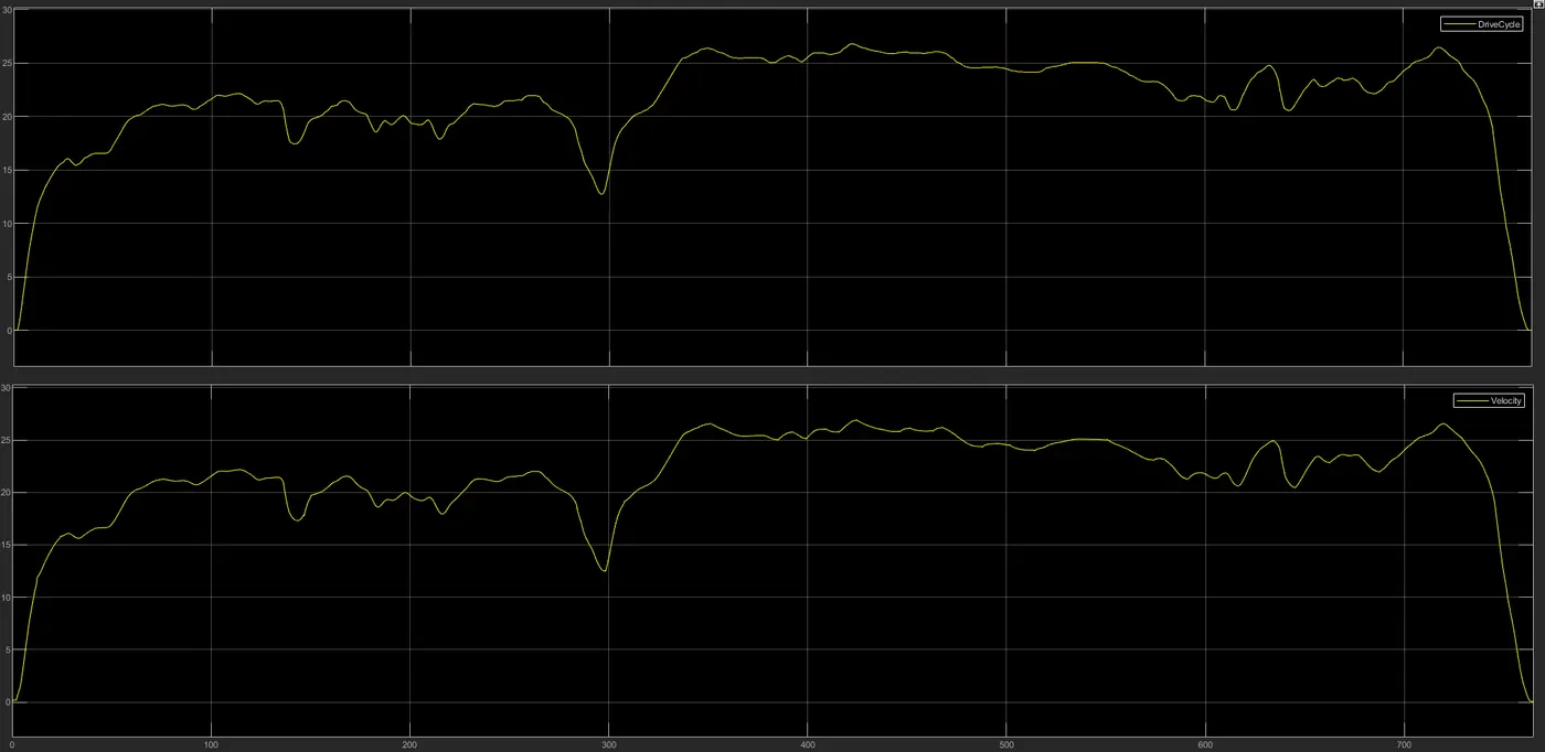
The velocity and drive cycle graph is shown above. They should be similar flowing graphs which they are after output.
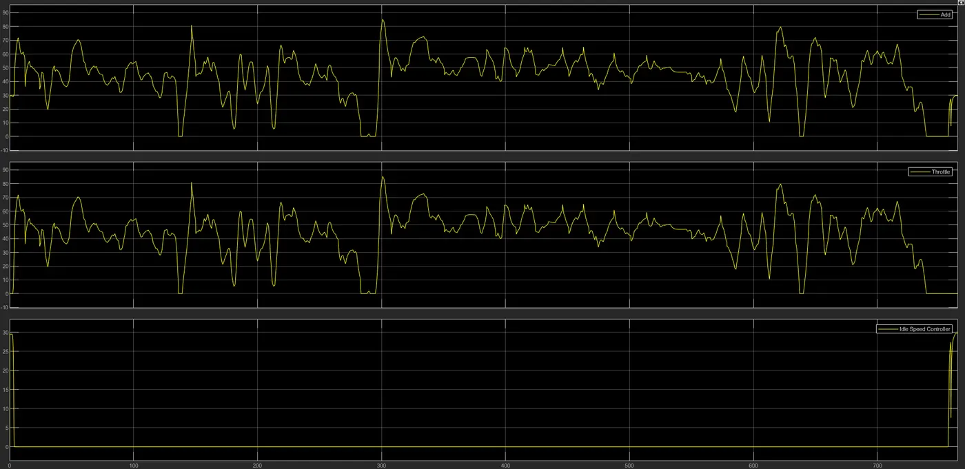
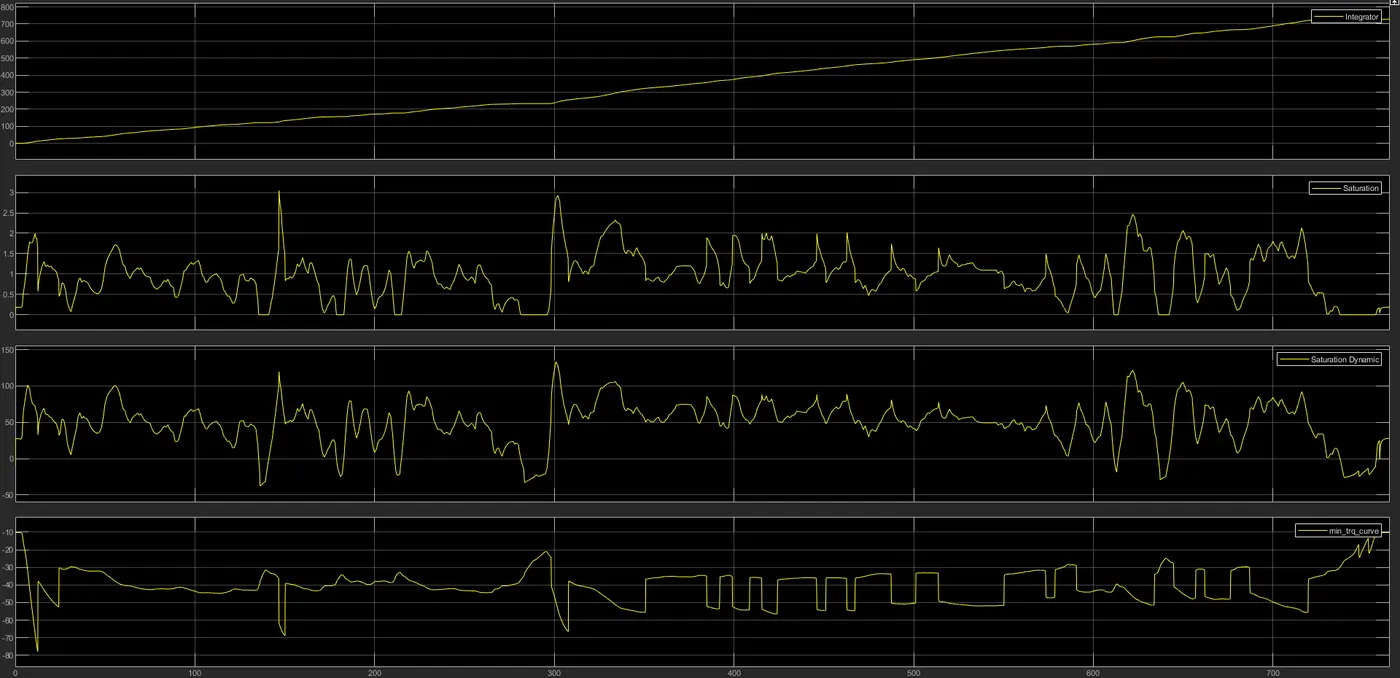
here, saturation is the engine fuel to air ratio graph. intrgrator is the engine fuel consumption graph. dynamic saturation is the engine speed graph. We need more fuel to air ratio when the power output required is more or increasing. When this ratio is satisfied, the engine output follows a similar trends.
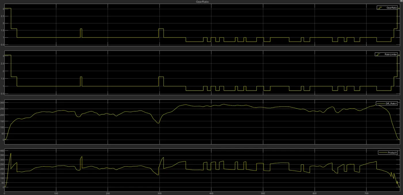
the gear ratio and rate limiter graphs are identical here. differential ratio and transitional speed are also output. in this model, we take engine torque, gear selector for transmission of gear ratio. the gear ratio is then multiplied by transmission input torque. This graph is seen in product1 and acts as transmission input speed. torque converter connects the engine to transmission.
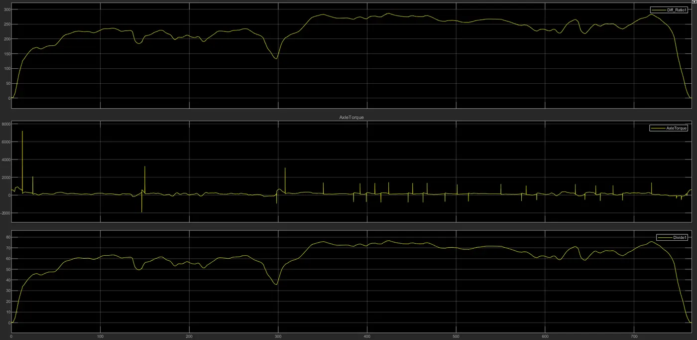
the above graphs shows transmission output speed, axle torque and wheel speed. the wheel and output speed have similar graphs. the axle torque acts whenever there is a change in the wheel speed.
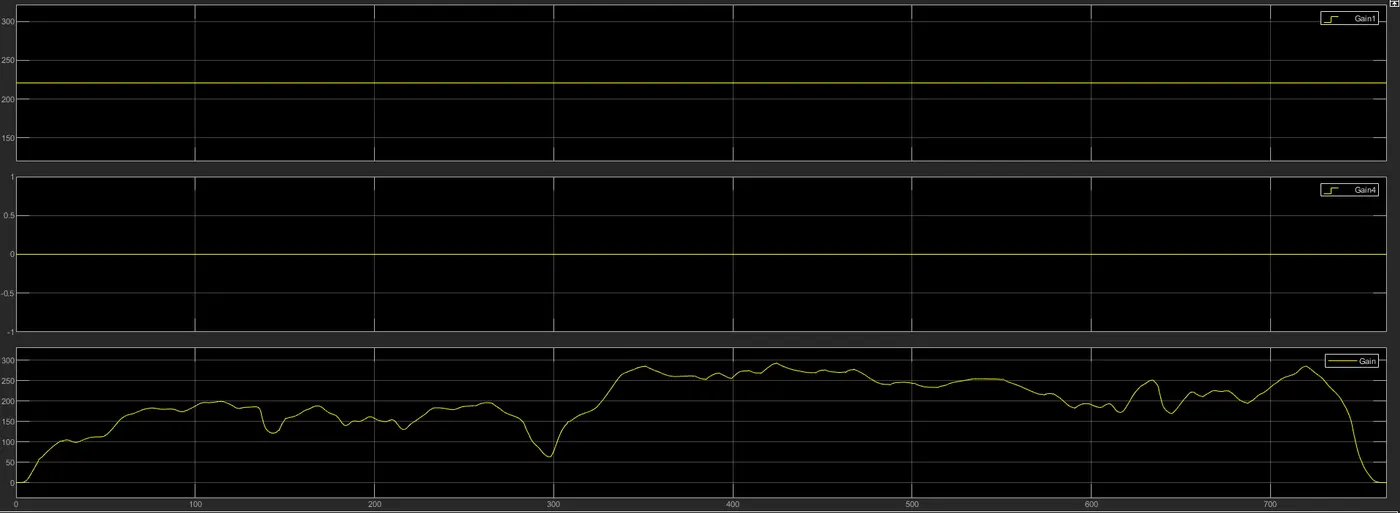
gain1 is constant rolling resistance force as theta is 0 degrees.
gain4 is grading force as theta is 0 degrees.
gain is the aerodynamic force which changes according to the velocity of vehicle.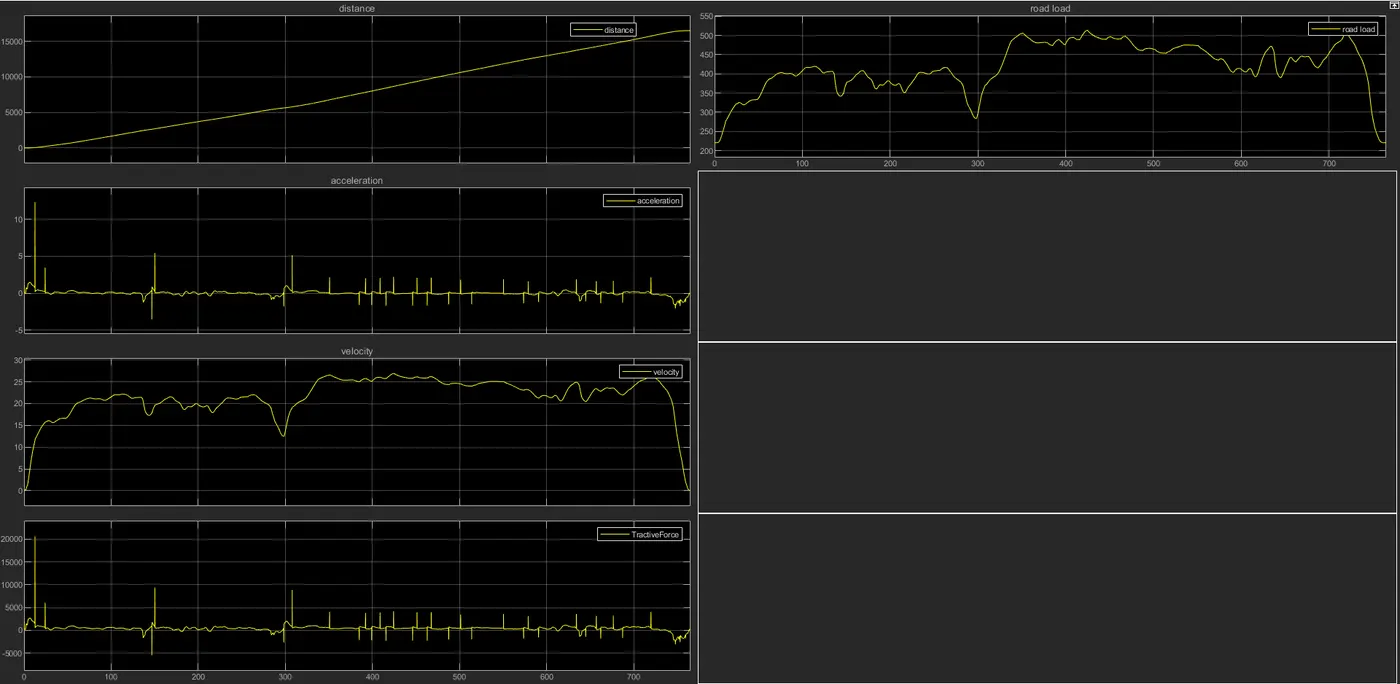
these is the distance, acc, vel, tractive force, road load graphs. Tractive force and acceleration have similar graphs. The distance goes on increasing irrespective of force or load conditions as the vehicle keeps on moving forward.