Parsing a file containing Thermodynamic Data using Matlab

Aim:

To extract the thermodynamic data (coefficients) for individual species, from a file and plot the variation of Specific Heat, Enthalpy, and Entropy in separate folders for each of them.

Theory:

File parsing refers to reading from a text file and creating a storing the data in such a way that it can be read, and operated upon to get useful information. Matlab can import many types of files, for example: text(CSV, TXT) spreadsheets( XLX, XLSX, XLSM etc), image data (BMP, JPG, JPEG etc) and many more.

In this particular exercise, we would be reading from a file with ‘.dat’ as its file extension.

This file is basically the thermodynamic data for different gases. The data is actually 14 coefficients for each individual gas, along with the local temperature ranges for which the coefficients hold true. With the use of these coefficients, one can find the values of Specific Heat, Enthalpy, and Entropy for an arbitrary number of values between the minimum and maximum temperatures in the local temp range of that specific gas. It is important to note, that along with the local temperature range, we also have to extract the average temp or intermediate temp. For all the temperatures below the average temperature, we have to use a different set of coefficients as compared to temperatures higher than the average temperature.

An image of the thermodynamic data file can be seen here:

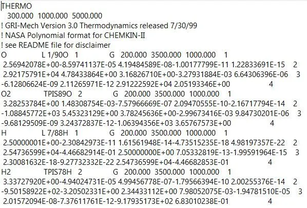
As we can see, there is header information consisting of the first 5 lines where in the first line is just the word THERMO. The second line is the Global Temperature Range and the next three lines include some other information that is not relevant for the sake of this assignment.

We now have to develop an algorithm to extract the coefficients in a stepwise and logical manner.

Algorithm for Data Extraction (Code Explanation) along with the code:

Before that, we need to have some basic idea of how we extract a line. We can use the fgetl() command to get the next line in a particular file. If we use the fgetl() command again, we get the immediate next line to one we previously got. We can use this property to extract sequentially, the required lines for each gas. Further it is important to note, that for each gas, we have one title line consisting the gas name, the local temp range and then three lines next to it which contain 14 coefficients, 5 in the first 2 and 4 in the 3^rd.

Note: When we say ‘extract a line using fgetl()’ , we get the’ location or pointer pointing to a line’ and store it in a variable

1. Open the THERMO file by using the fopen() command , with read (‘r’) mode.
2. Now extract the first line
3. Extract the second line of the global temperature range and using str2double() command, convert it to an array of numbers.
4. Extract the next three lines because they are irrelevant for the current project.
5. Now we start extracting individual species data:
6. For i = 1:53, do the following:
7. Use fgetl() to get the header of the first gas and store it in some variable. Use the strsplit() or splitstr() method and pass the delimiter as (‘ ‘) i.e, a space or blank. This will split the line whenever a space is encountered and then store this to another variable. This variable will automatically be of cell type. From the first cell, using extract the gas name and store it in a variable.

• Extract the data in (n-1)th, (n-2)th and (n-3)rd cells by using str2double and using {} around the index postions. This will convert the cell type data to normal string data. Do this for local average, local minimum, and local maximum temperatures. We now have the local temperature range for the first gas.

1. Create a separate array called ‘temp’ or any suitable name which will basically divide the local low and high temperatures, and create 500 values of temperatures including these two also.
2. Now get the next line, and using put A = strfind() method, obtain an array of values where the letter ‘E’ is stored. This array is naturally stored in a itself.
3. For the next three lines do the following:
4. Get the position of the first E. Get the characters from start of the line till E+3^rd index value and store it in a1. This will be the first coefficient.
5. For the second coefficient, extract the values from 4^th place after the first E till 3^rd place after the second E. This is a2, the second coefficient
6. Now repeat this process for all remaining coefficients

• We will now have all the 14 coefficients
• Calculate the cp, h, and s values for the current gas, by passing all the coefficients, temp array and the value of universal gas constant, in the respective functions for cp, h and s.

1. In the current working directory, create another directory with its name as the ‘species name’ which we have extracted in step ‘i’. For this, use the mkdir() function and pass the species name as a parameter.
2. Use the cd() function by passing the species name again as the parameter. This will change the location or pointer of current working directory, to the newly created directory for the specific gas.
3. Now plot the variation of cp vs T, h vs T, and s vs T for the current gas and save all the three files using the saveas() command and passing the figure handle and the name. These images will automatically be saved in the directory specially created for the gas.

• Now calculate the molecular weight of the gas by using a function and print it to the console window.
• Change the pointer to current working directory, back to the main directory by using cd . . command.

Formulae:

We also need to create functions to calculate the cp, h, and s for 500 temp values. The formulae for the same are:

For Specific Heat: (t = temperature in Kelvins)

Low Temp Range: cp = R*(a1 + a2*t + a3*t^2 + a4*t^3 + a5*t^4);

High Temp Range: cp = R*(a8 + a9*t + a10*t^2 + a11*t^3 + a12*t^4);

For Enthalpy: (t = temperature in Kelvins)

Low Temp Range: h = R*(a1 + a2*(t/2) + a3*(t^2/3) + a4*(t^3/4) + a5*(t^4/5) + a6/t);

High Temp Range: h = R*(a8 + a9*(t/2) + a10*(t^2/3) + a11*(t^3/4) + a12*(t^4/5) + a13/t);

For Entropy: (t = temperature in Kelvins)

Low Temp Range: s= R*(a1*log(t) + a2*t + a3*(t^2/2) + a4*(t^3/3) + a5*(t^4/4) + a7);

High Temp Range: s = R*(a8*log(t) + a9*t + a10*(t^2/2) + a11*(t^3/3) + a12*(t^4/4) + a14);

[Note: a1 to a7 are low temp coefficients and a8 to a14 are the corresponding high temp coefficients]

Therefore, for low temp range, we use a1 to a8 and for high temp range, we use a8 to a14.

Main Code:

clear all
close all
clc
%%
therm =  fopen('THERMO.dat','r');        % Open the file and create a file handle
a = fgetl(therm);                        % Extract the first line 
gtr = fgetl(therm);                      % Extract the global temperature range and store it n a variable 
gtr = str2double(gtr);                      % Convert the global temp range from string format to num format                                     
% k = fgetl(therm);
%%
for i = 1:3
    k = fgetl(therm);
end
 
%%
for i = 1:53
    % Extracting the information like gas name, local temperature range
    k = fgetl(therm);
    gas_data = strsplit(k,' ');
    gas_name = gas_data{1};
    
    local_avg_temp = str2double(gas_data{end-1});
    local_high_temp = str2double(gas_data{end-2});
    local_min_temp = str2double(gas_data{end-3});
    temp = linspace(local_min_temp,local_high_temp,500);
    
    %Extracting the first five coefficients:
    k = fgetl(therm);                     % Extract the first line of coefficients
    A = strfind(k,'E');                   % Find the positions where we have E
    
    %Based on the position where E is located, we read the coefficients 
    a1 = str2double(k(1:(A(1)+3)));
    a2 = str2double(k(A(1)+4:A(2)+3));
    a3 = str2double(k(A(2)+4:A(3)+3));
    a4 = str2double(k(A(3)+4:A(4)+3));
    a5 = str2double(k(A(4)+4:A(5)+3));
    
    %Extracting the next five coefficients:
    k = fgetl(therm);                     % Extract the next line of coefficients
    A = findstr(k,'E');
    
    a6 = str2double(k(1:(A(1)+3)));
    a7 = str2double(k(A(1)+4:A(2)+3));
    a8 = str2double(k(A(2)+4:A(3)+3));
    a9 = str2double(k(A(3)+4:A(4)+3));
    a10 = str2double(k(A(4)+4:A(5)+3));
     
    %Extracting the last four coefficients:
    k = fgetl(therm);                      
    A = findstr(k,'E');
    
    a11 = str2double(k(1:(A(1)+3)));          
    a12 = str2double(k(A(1)+4:A(2)+3));
    a13 = str2double(k(A(2)+4:A(3)+3));
    a14 = str2double(k(A(3)+4:A(4)+3));
   
 
    
    %Now calculate the Specific Heat, Specific Enthalpy, and Specific
    %Entropy for each gas
    R = 8.314;                            % Units = kJ/k-molK Universal gas constant
    cp = specific_heat(a1,a2,a3,a4,a5,a6,a7,a8,a9,a10,a11,a12,a13,a14,R,temp);
    h = specific_enthalpy(a1,a2,a3,a4,a5,a6,a7,a8,a9,a10,a11,a12,a13,a14,R,temp);
    s = specific_entropy(a1,a2,a3,a4,a5,a6,a7,a8,a9,a10,a11,a12,a13,a14,R,temp);
    
    
    mkdir(gas_name)
    cd(gas_name)
    
    figure(1)                             % Creating a figure handle
    plot(temp,cp);                        % Plotting the data
    xlabel('Temperature in Kelvins');
    ylabel('Specific Heat');
    title(['Specific Heat vs Temperature for: ',gas_name]);
    saveas(figure(1),'Specific Heat vs Temperature.jpg');    %saving the figure to the current directory
    
    figure(2)
    plot(temp,h);
    xlabel('Temperature in Kelvins');
    ylabel('Enthalpy');
    title(['Enthalpy vs Temperature for: ',gas_name]); 
    saveas(figure(2),'Enthalpy vs Temperature.jpg');
    
    figure(3)
    plot(temp,s);
    xlabel('Temperature in Kelvins');
    ylabel('Entropy');
    title(['Entropy vs Temperature for: ',gas_name]);
    saveas(figure(3),'Entropy vs Temperature.jpg');
   
    M = molecular_weight(gas_name);                         %calculating molecular weights
    fprintf('Molecular weight of %s is:n',gas_name);
    disp(M);
 
cd ..           %shifting the current directory address, back to the original main directory
    
 
end

Code for Specific Heat:

function [output] = specific_heat(a1,a2,a3,a4,a5,a6,a7,a8,a9,a10,a11,a12,a13,a14,R,temp)
 
for i = 1:length(temp)
   
    t = temp(i);
    cp(i) = R*(a1 + a2*t + a3*t^2 + a4*t^3 + a5*t^4);
    if t>1000
        cp(i) = R*(a8 + a9*t + a10*t^2 + a11*t^3 + a12*t^4);
    end
 
[output] = cp;
end

Code for Enthalpy:

function [output] = specific_enthalpy(a1,a2,a3,a4,a5,a6,a7,a8,a9,a10,a11,a12,a13,a14,R,temp)
for i = 1:length(temp)
   
    t = temp(i);
    h(i) = R*(a1 + a2*(t/2) + a3*(t^2/3) + a4*(t^3/4) + a5*(t^4/5) + a6/t);
    if t>1000
        h(i) = R*(a8 + a9*(t/2) + a10*(t^2/3) + a11*(t^3/4) + a12*(t^4/5) + a13/t);
    end
 
[output] = h;
end

Code for Entropy:

function [output] = specific_entropy(a1,a2,a3,a4,a5,a6,a7,a8,a9,a10,a11,a12,a13,a14,R,temp)
for i = 1:length(temp)
    
    t = temp(i);
    s(i) = R*(a1*log(t) + a2*t + a3*(t^2/2) + a4*(t^3/3) + a5*(t^4/4) + a7);
    if t>1000
        s(i) = R*(a8*log(t) + a9*t + a10*(t^2/2) + a11*(t^3/3) + a12*(t^4/4) + a14);
    end
 
[output] = s;
end

Code for Molecular Weight:

function output = molecular_weight(gas_name)
elements = ['C','H','O','N','S','AR'];
mw = [12.011,1.008,15.999,14.007,32,39.948];
weight = 0.00;
temp = 0;
counter = 0;
for i = 1:length(gas_name)
    for j = 1:length(elements)    
          if strcmp(gas_name(i),elements(j))==1
              weight = weight + mw(j);
              temp = j;
          end
    end
    counter = str2double(gas_name(i));
    if counter >1
        weight= weight + mw(temp)*(counter-1);
    end
               
output = weight;
end

Observation:

• The values of cp, h, s vs T are plotted.
• These values vary drastically for all the gases.

Some randomly selected graphs are shown here:

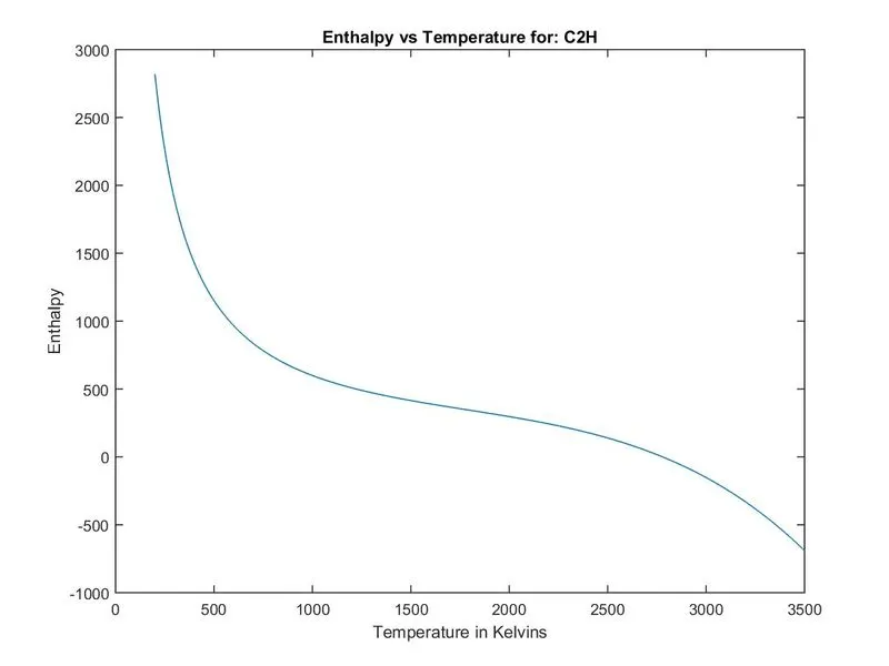
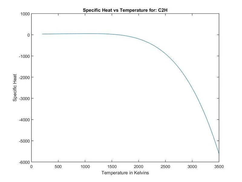
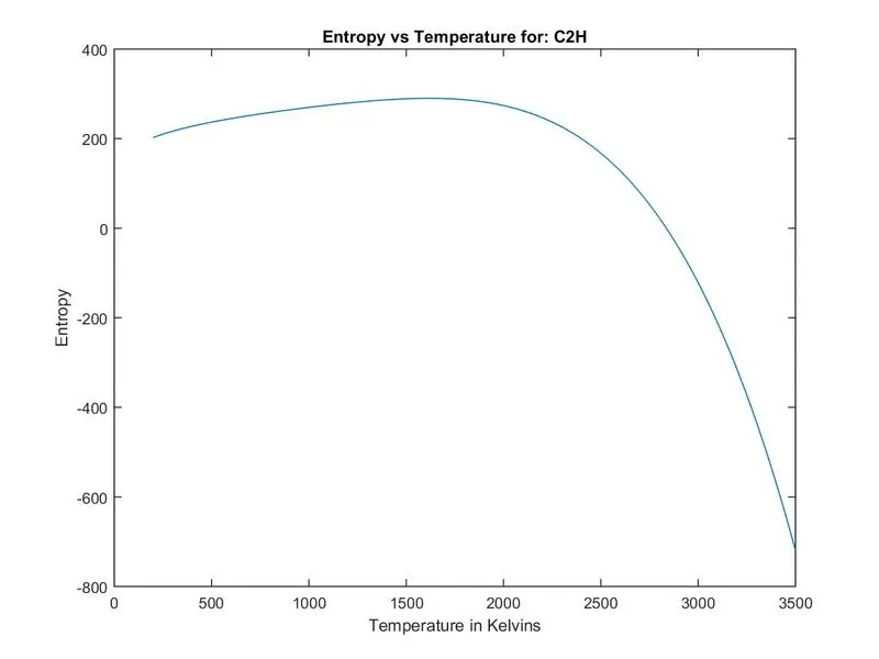
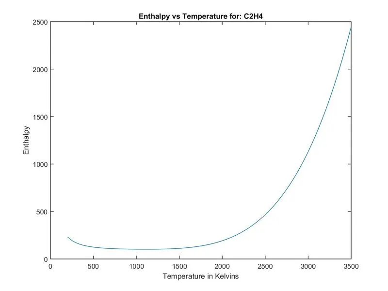
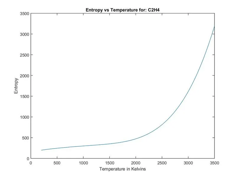
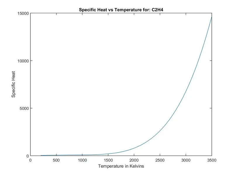
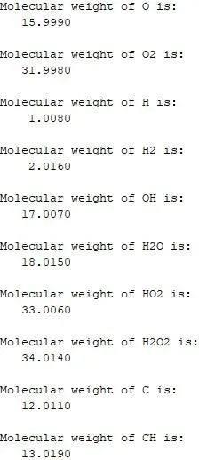
The command window at the end of the execution shows the molecular weight for each gas:

Conclusion:

The file parsing was thus successfully completed. The thermodynamic coefficients were properly extracted and the atomic weights were also printed. For lengthier files and more complicated datasets, we need more rigorous algorithms.