SIMULATING THE MOTION OF A SIMPLE PENDULUM IN MATLAB

REPORT:

AIM:

1. To solve the second order governing differential equation (GDE) for damped oscillations of a pendulum using Matlab.
2. To plot angular displacement and angular velocity vs time.
3. To create a movie/animation in Matlab, showing the time varying oscillations of the simple pendulum.

THEORY:

The governing differential equation for a simple pendulum with damped oscillations is:

d2(theta)/dt2 + (b/m)*d(theta)/dt + (g/L)*sin(theta) = 0

In the above equation,

t = time (seconds)

b = damping coefficient (Nm/sec)

m = mass of the pendulum bob (kg)

(theta) = angular displacement (radians)

d(theta)/dt = angular velocity (radians/sec)

d²(theta)/dt² = angular acceleration (radians/sec²)

L = length of the pendulum (meters)

• The difference between an undamped free oscillation and a damped free oscillation is, in the undamped case, the oscillation continues infinitely whereas in the damped case, the amplitude of the oscillation decays with time and gets closer and closer to zero.
• After solving the second order differential equation, the outputs would be an equation for angular displacement and an equation for velocity.
• The initial conditions are: at time = 0, theta = 0 and angular velocity = 5 rad/sec
• Matlab takes these initial conditions, solves the differential equation by numerical integration (Runge- Kutta method) and gives an output.
• Numerical integration gives an output array instead of a single numerical output.
• The function/command used to solve the GDE is
• The syntax for ode45 command is:

[output] = ode45(@(inputs) function_name(parameters), independent_variables, initial_conditions)

• Also, an important point to note here is, that we are breaking the original second order differential equation into two first order equations, because the solver ode45 can only work on first order equations.
• The two first order equations are described in the formulae section.

FORMULAE:

Apart from the above differential equation, the formulae defining the cartesian co-ordinates needed for plotting the pendulum’s time varying motion are:

1. Formulae for function definition:

Let us replace theta in the original equation by theta1

d(theta1)/dt = theta2

d(theta2)/dt = (-b/m)*theta2 – (g/L)*sin(theta1)

2. Formulae for creating the animation:

x0 = any user defined value (x co-ordinate of the fixed end of string)

y0 = any user defined value (y co-ordinate of the fixed end of string)

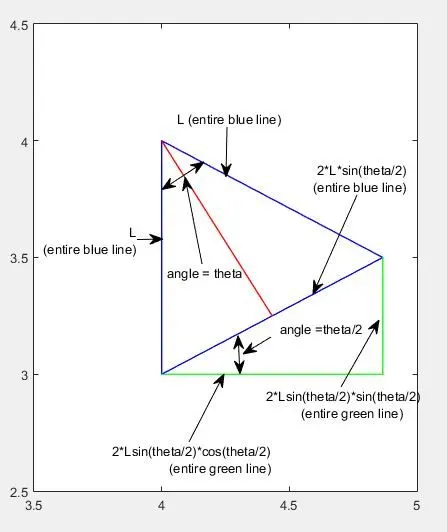
x1 = x0 + L*sin(theta) (x co-ordinate of the free end of string)

y1 = (y0-L) + 2L*sin²(theta/2) (y co-ordinate of the free end of string)

[The following graph shows the diagram through which we arrive at the above formulae. The two blue lines with text arrows showing 'L', depict the pendulum string positions. Other lines depict the construction lines. The point (4,4) is the point of suspension.]

GRAPHICAL PROOF OF THE FORMULAE:

COUNTERS AND TERMINOLOGIES USED IN THE CODE ALGORITHM:

Before describing the code algorithm/explanation, some important counters need to be defined.

• ct = frame counter. This counter increases, each time a new frame is plotted. According to the value of ct, the array M stores the latest displayed frame, into an index position equal to the latest value of ct.
• i = angular position indicator. This counter increases, after a definite pause, and the value of ‘i’, denotes the index of the new value of displacement theta, in the first column of results.
• tspan = an array with initial value of time and final value of time.
• size of tspan = number of steps taken to reach the final value of tspan.(i.e, the size of the array tspan)
• displacement column = first column in the array of results which denotes angular displacement.

PROCEDURE/CODE EXPLANATION:

The logic flow/ algorithm for the code is:

1. Input the range and step-size for the independent variable in this case, the time span of integration.
2. Define the initial conditions.
3. Define an output array in this case [t, results] and equate it to the ode45 function call.
4. Plot results vs time to obtain the graphical representation of displacement and velocity variation w.r.to time.
5. Initiate ct = 1
6. Initiate i = 1
7. Declare x0, y0, x1, y1, length L
8. Intake the instantaneous value of theta from the first column of ‘results’ array (displacement column).
9. Plot a line joining [x0 y0] and [x1 y1] and plot the pendulum bob at x1, y1 using the geometric relations including theta.
10. Set the axes appropriately.
11. Pause for [(final value of tspan – initial value of tspan) /size of tspan] seconds.
12. Create and array M(ct) and in it, attach the current figure at the index position defined by ct.
13. ct = ct +1
14. If i = size of displacement column, go to step 15 else go to step 7.
15. Create a movie of the array M
16. Create a new video file and give it a suitable name.
17. Open the new video file and write the information stored in array M into it.
18. Close the video file.

[Please note: In the above code-explanation, step 5 which plots the graph of displacement and velocity variation with respect to time, it is more beneficial that the graph be plotted in a separate code or else it will interfere with the pendulum animation. Also, the algorithm for the ode function is explained in descriptive form in the general explanation below.]

General explanation of the code:

The solver takes the input values of time and initial angular velocity. It first integrates d(theta1)/dt, w.r.to time, and stores that value into first section of 'results' array, which denotes angular displacement. It then takes the integral of d(theta2)/dt or in other words, the double integration of d²(theta1)/dt², and stores that in the second column of 'results' array which denotes the angular velocity. The time step now increases and the same process is done for the latest values of integrates d(theta1)/dt and d(theta2)/dt. After the integration is complete, the 'results' array is updated.

CODE:

The code for plotting the graph of displacement-velocity vs time is:

clear all 
close all
clc
%Defining the initial conditions for angular position and velocity
theta_initial = [0;3];
%defining the constants in the differential equation
b = 0.05;                 %damping constant, units(Nm/sec)
g = 9.81;                 %gravitational acceleration, units(m/sec^2)
l = 1;                    %length of the pendulum units(m)
m = 0.1;                  %mass of the pendulum units(kg)
%t_span indicates the time span for integration
t_span = linspace(0,20,600);
 
[t,results] = ode45(@(t,theta) ode_func(t,theta,b,g,l,m),t_span,theta_initial);
plot(t,results(:,1))
hold on 
plot(t,results(:,2))
xlabel('Time');
ylabel('Plot');

The code for creating the animation is:

clear all 
close all
clc
 
%defining the constants in the differential equation
b = 0.05;                 %damping constant, units(Nm/sec)
g = 9.81;                 %gravitational acceleration, units(m/sec^2)
l = 1;                    %length of the pendulum units(m)
m = 0.1;                  %mass of the pendulum units(kg)
 
%Defining the initial conditions for angular position and velocity
theta_initial = [0;3];
 
%t_span indicates the time span for integration
t_span = linspace(0,20,600);
 
[t,results] = ode45(@(t,theta) ode_func(t,theta,b,g,l,m),t_span,theta_initial);
%creating the animaion
ct = 1;                    %initiating the frame counter
for i = 1:length(t_span)   %initiating the angular position counter
    instantaneous_theta = results(i,1);
    l = 1;
    x0 = 4;
    y0 = 4;
    %calculating the co-ordiantes of free end of the string
    x1 = 4+l*sin(instantaneous_theta);
    y1 = (4-l)+2*l*(sin(instantaneous_theta/2)^2);
    %plotting the string and the pendulum bob
    plot([x0 x1],[y0 y1],'linewidth',1,'color','blue'); 
    hold on 
    plot(x1,y1,'.','MarkerSize',50,'color','red');
    hold off
    axis([3 5 2 4]);
    set(0,'defaultfigureposition',[100 100 655 600]) %setting the frame to a fixed size
    pause(t_span/600); 
    M(ct)= getframe(gcf);
    ct = ct+1;
end 
 movie(M);
 videofile = VideoWriter('Simple_Pendulum.avi','Uncompressed AVI');
 open(videofile);
 writeVideo(videofile,M);
 close(videofile);

RESULTS:

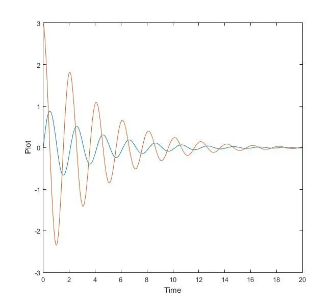
The result in the form of graph is attached below:

In the grapg below, Red colored plot = Angular Velocity

Blue colored plot = Angular Displacement

CONCLUSION:

1. The graph obtained for the angular position and angular velocity vs time proves that the more is the value of the damping coefficient(constant) ‘b’, the faster the oscillation decreases in amplitude.
2. The exponential decay of the graph is due to the damping whereas the sinusoidal nature is due to the oscillation.
3. If the damping coefficient exceeds the value of critical damping coefficient, the system becomes overdamped and if it becomes equal to critical damping coefficient, the system becomes critically damped.