Using Genetic Algorithm to maximize a given function

Aim: To implement Genetic Algorithm for maximization of the given function

Theory:

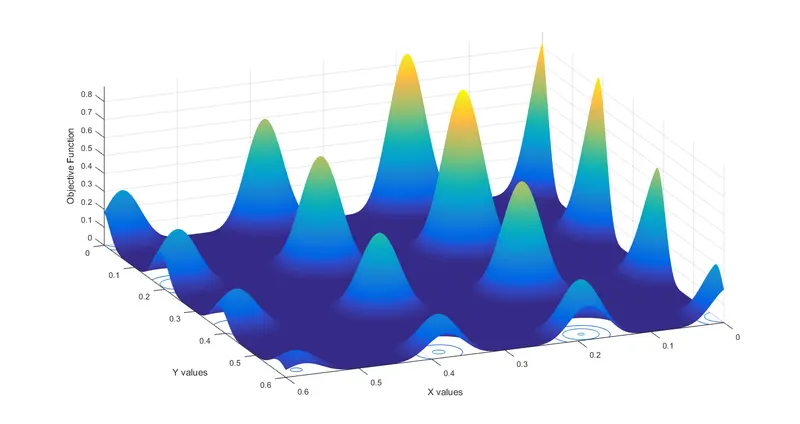
The above 3D image is that of the function which we are using in this project

Genetic algorithm has its roots in the Darwin’s theory of evolution, or in other words, survival of the fittest. This approach mimics the concept of evolution. The base idea is that evolution is analogous to an ‘Optimization Process’. What we optimize, is some objective function which may depend on one or more variables. Each generation in evolution corresponds to an ‘iteration’ in genetic algorithm. Biological systems are more robust and have the capability of recreation and also self-repair. However, the most important property is that of adapting to external changes, by modifying the genetics themselves. While traditional optimization algorithms can converge to local maxima or minima, a global optimization algorithm will always converge to the global minima or maxima. The differences between a genetic algorithm (GA), and conventional optimization techniques are:

• In GA, every variable is associated with a code (generally, a binary code) and not with the absolute value of the independent variables.
• GA s work with multiple points, not just one point.
• GA s do not use the first or second derivative information. Instead, they directly use the value of the objective function themselves.
• GA s use stochastic (probabilistic transition rules) and not deterministic rules.

How does the GA work?

1. If we have n number of independent variables, then we choose 2n to 4n number of trial solutions. Note that trial solutions are nothing but values of independent variables themselves.
2. We represent each trial solution by a string of binary variables (1’s and 0’s). These strings, correspond to chromosomes in biological systems.
3. If we need higher accuracy (i.e., more decimals), we can add a greater number of decimal places and increase the corresponding string length. The value of the objective function evaluated at any particular trial solution, will be analogous to the concept of ‘fitness of survival’ in terms of genetics. However, depending on whether we are dealing with minimization or maximization problems, we can measure fitness by either maximum or minimum value of objective function.
4. Then, we use stochastic techniques to produce child strings, i.e, new values for trial solutions, by using crossover techniques which also occur in chromosomes. Suppose we have ‘n’ solutions in the first iteration. We evaluated the value of objective function for all of them, and found out that for some ‘k’ number of trial solutions, the objective function is either too low, or too high (depending on whether it is minimization or maximization problem). Thus, we will eliminate those k values and will be left with ‘n-k’ trial solutions in the mating pool for the first iteration. Mating pool is just the set of trial solutions which are fit to produce children. Now, these ‘n-k’ trial solutions of the first iteration have become ‘parents’ for the second iteration and will perform binary crossovers and mutations to produce n-k children (even if two chromosomes come together to produce a child, crossover effects both the parent chromosomes, thus we get two children). If we are dealing with constant population GA, then we need to make ‘k’ copies of the fittest parent in the mating pool of first generation, to compensate for the k values which we removed. In this case, we will always have ‘n’ children in each iteration in a constant population approach.
5. What is mutation? Well, there is a difference between crossover and mutation. Crossover happens ‘two’ parent chromosomes (in our case, two binary strings), exchange bits at some corresponding positions, where as in mutation, some randomly bits in one single string are flipped (1 is changed to 0 and vice versa). Mutation is done, because if we keep on performing crossovers with the fittest parent, it may so happen that in some iteration, some desired characteristics of the fittest parent will be lost, that is, they won’t be passed on to the child string. To avoid this, we flip some bits randomly.

Matlab Code and its explanation (Alongwith the syntax for GA solver):

The step-wise explanation of matlab code is as follows:

• Input the x and y vectors
• With the help of meshgrid, create a matrix with xx and yy values
• Evaluate the value of the Stalagmite function for each point in the meshgrid and store it in an array
• Create a surface plot to visualize the surface of the function.
• Now run the genetic algorithm code. It is important to note that if we do not provide lower and upper bounds to the solver, then we will get extremely different solution each time. To pass the lower and upper bounds, we basically do the following:

[solution,fval,exitflag,output,population,scores]=ga(FITNESSFCN,NVARS,A,b,Aeq,beq,lb,ub,NONLCON,options)

(Note: This syntax is directly taken from matlab help section)

1. solution = a 1 by 2 array with the x and y values for which we get the global maximum.
2. fval = computes maximum value of the function

• exitflag = gives the exit condition of the GA

1. output is basically a structure with attributes like generation, function count, maximum constraints and a message
2. population = the population at the end of GA termination.
3. scores = returns the scores of the final population

• FITNESSFCN = The fitness function which in our case, is the stalagmite function
• NVARS = number of variables = 2

1. A = put []
2. B = put []
3. Aeq = put []

• Beq = put []
• Lb = (lower bounds for the independent variables) [0 0] (or put any other value that is needed)
• Ub = (lower bounds for the independent variables) [0.6 0.6] (or put any other value that is needed)
• NONLCON = nonlinear constraints = put [] because we do not have any nonlinear constraints like a circular search region or any other shape

• Options = enter options from the ‘optimset’ function.

According to above syntax, we define our GA function as:

[solution,fval,exitflag,output,population,scores] = ga(@stalagmite,2,[],[],[],[],[0 0],[0.6 0.6],[],[],options);

Here,

options = gaoptimset('PlotFcn’,@gaplotbestf,'PlotInterval',1,'PopulationSize',50);

The main code for GA is:

clear all
close all
clc
 
x = linspace(0,0.6,600);
y = linspace(0,0.6,600);
 
[xx,yy] = meshgrid(x,y);
 
for i = 1:length(xx)
    for j = 1:length(yy)
        input_vector(1) = xx(i,j);
        input_vector(2) = yy(i,j);
        f(i,j) = stalagmite(input_vector);     
    end   
end
 
surfc(xx,yy,-f);
xlabel('X values');
ylabel('Y values');
zlabel('Objective Function');
 
shading interp
 
options = gaoptimset('PlotFcn',@gaplotbestf,'PlotInterval',1,'PopulationSize',50);
 
[solution,fval,exitflag,output,population,scores] = ga(@stalagmite,2,[],[],[],[],[0 0],[0.6 0.6],[],[],options);
 
fprintf('The maximum value of the function is: %7.6f',abs(fval));

The code for the function is:

function [output] = stalagmite(input_vector)
 
f1x = sin(5.1*pi*(input_vector(1) + 0.5)).^6;
f2x = exp(-4*log(2)* ((input_vector(1)-0.0667).^2/0.64));
f1y = sin(5.1*pi*(input_vector(2) + 0.5)).^6;
f2y =  exp(-4*log(2)* ((input_vector(2)-0.0667).^2/0.64));
 
f = (f1x*f2x*f1y*f2y);
 
[output] = -f;
end

Observations:

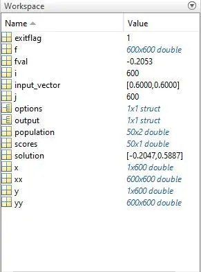
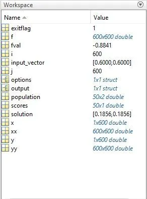
We observe that if we give unbounded constraints, then the solution will not always converge to the same value. However, with bounded constraints, the solution will always converge to the same value. This is clearly seen below.

In this image, the fval is extremely different than the maximum value present in the array of 'f' which is the function we need to minimize.

Note: Value is negative because we have defined stalagmite function in that manner

In this image, the fval is exactly equal to the maximum value present in the array of 'f' which is the function we need to minimize.

Similarly this can be observed in the graphs:

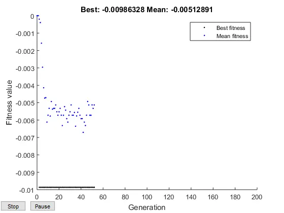
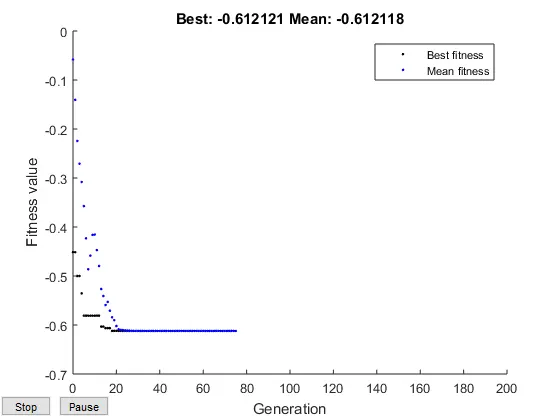
• Also, since the GA in Matlab is programmed for minimization, we need to multiply our original function with -1 to maximize it.

Conclusion:

• A genetic algorithm is useful when we have multiple objective functions and their combined minimization or maximization is cumbersome if done by calculus.
• The bounded approach will always give persistent results as compared to unbounded initial conditions.
• The genetic algorithm will stop, in two cases: the number of generations has reached its maximum limit, or the desired tolerance level is achieved.