Curve Fitting Using Matlab

Aim: To perform curve-fitting on the data for variation of specific heat with temperature

Theory:

• Curve Fitting and using the Split-wise Approach:

Curve fitting refers to the process of finding or generating a curve that passes through all or most of the data points in a given dataset. The most common method of curve fitting can be a polynomial interpolation, wherein we generate a polynomial with the given data, that best describes the nature of the dataset. This polynomial might not be totally accurate but will try to match the actual values of the dataset to great extent. The main advantage of having such a polynomial is that we can use it to find the value of the function/dependent variable for a specific value of the independent variable. This value can lie within the domain of the independent variable or also outside it.

We can express a given data set with n+1 data points, in terms of an n degree polynomial as:

a_nx_n ⁿ+ a_n-1x_n-1^n-1 + a_n-2x_n-2^n-2 + … a₀

In Matlab, we can use the polyfit command to generate the polynomial coefficients (a_n, a_n-1, …a₀). Then, by using the polyval command, we can calculate the value of this polynomial for every X-value.

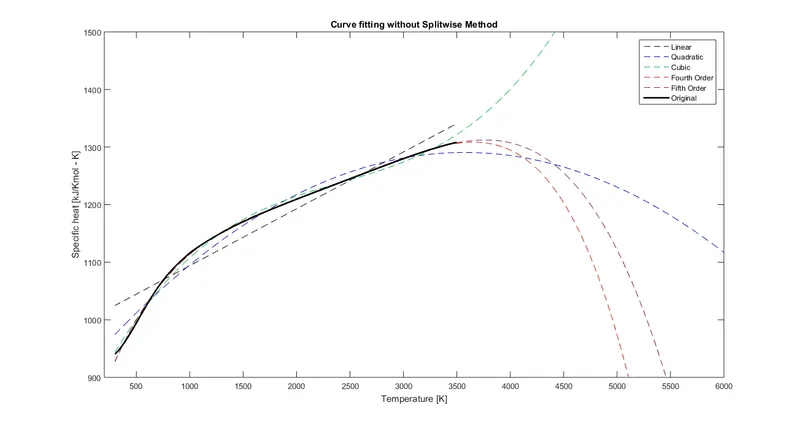
It is important to note that this curve fitting can be done is two ways: with and without splitting the data set. Incase we do not use split-wise method, that is to say we approximate the entire data set with one single polynomial, then this polynomial may approximate the curve initially, but can have major deviations for further values. If we divide this data in parts and create a separate polynomial for each, then these deviations/oscillations of the polynomial above and below the original curve can be minimized a lot.

• Errors and Coefficient of Determination (R-squared)

When fitting curve, errors are unavoidable because no line or polynomial can perfectly approximate the original curve. More scattered is the data, higher will be the errors. Also, errors can have both positive and negative values, thus we cannot just take the algebraic sum of all the errors and call it as the total error, because the addition of all positive errors and addition of negative errors may cancel each other out, although the individual errors are large. There are some measures to quantify these errors and find how much of a good fit, is the line or the curve.

Let mean of y = ӯ, each individual datapoint = y_i and y value of the predicted curve or line, be y

SSE or Sum of Squared Errors = Σ (y - y_i)²

SST or Sum of Squares Total = Σ (y_i - ӯ)²

SSR or Sum of Squares due to Regression = Σ (y - ӯ)²

Also, SST = SSR + SSE

R² or R squared is the coefficient of determination, which is:

R² = 1 – (SSE)/(SST)

R squared denotes ‘how much’ or ‘what fraction’ of the total variation (i.e SST), is explained by the regression line or curve (SSE) (or in other words, by the variation in x).

It can be observed that lower is the SSE, lower would be the ratio SSE/SST and hence, higher will be the value of R-squared. Thus, R-squared will get closer to 1, if SSE gets closer to 0.

Matlab Code:

The Matlab Code has been attached for the entire program. Along with a linear and cubic approximation, a Quadratic, Fourth and Fifth order approximation is also plotted for the non-split-wise method.

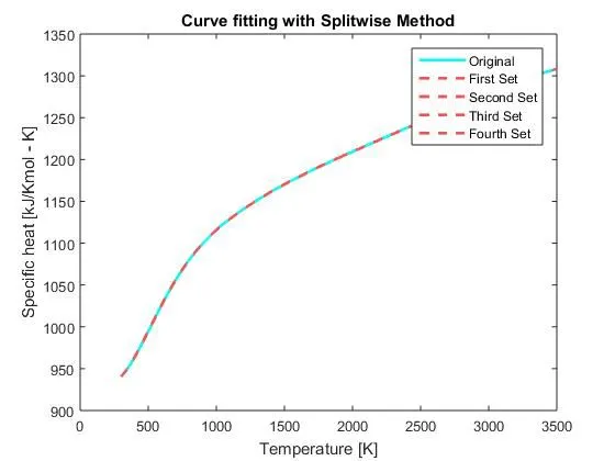
For the split-wise method, the data is split into four parts of 800 data points and a polynomial is fitted for each set. The order for every individual polynomial is accepted as a user's input. This allows the user to visualize how increasing or decreasing the order can change the accuracy of the fit.

For centering and scaling a polynomial, we use the following method:

We standardize the X data, by the formula ẋ = (x – mu(1))/(mu(2)), where mu(1) is the mean of x and mu(2) is the standard deviation of x. This standardization can be done by Matlab polyfit command itself. This helps in eliminating the centering and scaling errors.

[Note: The non-split-wise method is deliberately not centered and scaled to make the warnings visible. The centering and scaling are later applied only for the split-wise method.]

Code Explanation:

• Import the data file using the load command
• Extract temp and cp values in separate arrays
• Use the polyfit command to obtain polynomial coefficient value for each degree of polynomial and store these in a separate variable
• Use polyval command to plot the polynomial value for each temp value by uing the coefficients obtained in polyfit
• Calculate SSE by taking the difference between actual and interpolated cp for each cp value and squaring the sum of these errors
• Calculate SST by squaring the sum of differences between actual and average cp for each cp value
• Plot the data using plot command

close all
clc
%% Importing Data 
 
cp_data = load('data');
temp = cp_data(:,1);
cp = cp_data(:,2);
cp_mean = sum(cp)/length(cp);
extended_x = linspace(3500,6000,2500);
%% Potting original data set
 
plot(temp,cp,'linewidth',3,'color','cyan')
xlabel('Temperature [K]');
ylabel('Specific heat [kJ/Kmol - K]');
 
%% Fitting Polynomials for the entire dataset(quadratic,cubic,fourth order, fifth order)  
coeff_linear = polyfit(temp,cp,1);
coeff_quadratic = polyfit(temp,cp,2);
coeff_cubic = polyfit(temp,cp,3);
coeff_fourth = polyfit(temp,cp,4);
coeff_fifth = polyfit(temp,cp,5);
 
Line_Pred = polyval(coeff_linear,temp);
Quad_Pred = polyval(coeff_quadratic,temp);
Cube_Pred = polyval(coeff_cubic,temp);
Fourth_Pred = polyval(coeff_fourth,temp);
Fifth_Pred = polyval(coeff_fifth,temp);
 
Quad_Predx = polyval(coeff_quadratic,extended_x);
Cube_Predx = polyval(coeff_cubic,extended_x);
Fourth_Predx = polyval(coeff_fourth,extended_x);
Fifth_Predx = polyval(coeff_fifth,extended_x);
 
 
plot(temp,Line_Pred,'--','linewidth',0.5,'color','black')
hold on
plot(temp,Quad_Pred,'--','linewidth',0.5,'color',[0.0 0.0 0.75])
hold on
plot(temp,Cube_Pred,'--','linewidth',0.5,'color',[0.0 0.7 0.25])
hold on
plot(temp,Fourth_Pred,'--','linewidth',0.5,'color',[0.78 0.1 0.0])
hold on
plot(temp,Fifth_Pred,'--','linewidth',0.5,'color',[0.5 0.1 0.25])
hold on
plot(temp,cp,'linewidth',2,'color','black')
hold on
plot(extended_x,Quad_Predx,'--','linewidth',0.5,'color',[0.0 0.0 0.75])
hold on
plot(extended_x,Cube_Predx,'--','linewidth',0.5,'color',[0.0 0.7 0.25])
hold on
plot(extended_x,Fourth_Predx,'--','linewidth',0.5,'color',[0.78 0.1 0.0])
hold on
plot(extended_x,Fifth_Predx,'--','linewidth',0.5,'color',[0.5 0.1 0.25])
hold off
axis([200 6000 900 1500]);
title('Curve fitting without Splitwise Method');
legend('Linear','Quadratic','Cubic','Fourth Order','Fifth Order','Original');
xlabel('Temperature [K]');
ylabel('Specific heat [kJ/Kmol - K]');
 
%% Calculating errors and R-squared coefficients for all degrees
deviations = cp - cp_mean;
SST = sum(deviations.^2);
 
e1 = Line_Pred - cp;
SSE1 = sum(e1.^2);
 
e2 = Quad_Pred - cp;
SSE2 = sum(e2.^2);
 
e3 = Cube_Pred - cp;
SSE3 = sum(e3.^2);
 
e4 = Fourth_Pred - cp;
SSE4 = sum(e4.^2);
 
e5 = Fifth_Pred - cp;
SSE5 = sum(e5.^2);
 
rsq1 = 1 - SSE1/SST;
rsq2 = 1 - SSE2/SST;
rsq3 = 1 - SSE3/SST;
rsq4 = 1 - SSE4/SST;
rsq5 = 1 - SSE5/SST;
 
fprintf('nThe R-squared values for the non-splitwise-method polynomials are:nn');
fprintf('For Linear Fit: %7.6fn',rsq1);
fprintf('For Quadratic Fit: %7.6fn',rsq2);
fprintf('For Cubic Fit: %7.6fn',rsq3);
fprintf('For Fourth Order Fit: %7.6fn',rsq4);
fprintf('ForFifth Order Fit: %7.6fnn',rsq5);
 
%% Taking a user input to select order for indivisual polynomials
disp('To select the order of the approximating polynomial, enter an integer between 2 and 5');
k = [];
k(1) = input('Order of polynomial for set 1: ');
k(2) = input('Order of polynomial for set 2: ');
k(3) = input('Order of polynomial for set 3: ');
k(4) = input('Order of polynomial for set 4: ');
 
plot(temp,cp,'linewidth',2,'color','cyan')
title('Curve fitting with Splitwise Method');
xlabel('Temperature [K]');
ylabel('Specific heat [kJ/Kmol - K]');
 
hold on
 
for i = 1:4
    a = (1+800*(i-1));
    b = 800*i;
   
    if k(i)==2
        [coeff_quad,S1,mu1] = polyfit(temp(a:b),cp(a:b),2);
        Quad_Predxi = polyval(coeff_quad,temp(a:b),S1,mu1);
        plot(temp(a:b),Quad_Predxi,'--','linewidth',2,'color',[1 0 0]);
        d1 = deviations(a:b);
        sst1 = sum(d1.^2);
        es1 = Quad_Predxi - cp(a:b);
        sse1 = sum(es1.^2);
        r21 = 1 - sse1/sst1;
        fprintf('nFor the Quadratic curve, the R-squared value is: %7.6fn',r21);
        hold on
     elseif k(i)==3
        [coeff_cube,S2,mu2] = polyfit(temp(a:b),cp(a:b),3); 
        Cube_Predxi = polyval(coeff_cube,temp(a:b),S2,mu2);
        plot(temp(a:b),Cube_Predxi,'--','linewidth',2,'color',[0 1 0]);
        d2 = deviations(a:b);
        sst2 = sum(d2.^2);
        es2 = Cube_Predxi - cp(a:b);
        sse2 = sum(es2.^2);
        r22 = 1 - sse2/sst2;
        fprintf('For the Cubic curve, the R-squared value is: %7.6fn',r22);
        hold on
     elseif k(i)== 4
        [coeff_fourth,S3,mu3] = polyfit(temp(a:b),cp(a:b),4);  
        Fourth_Predxi = polyval(coeff_fourth,temp(a:b),S3,mu3);
        plot(temp(a:b),Fourth_Predxi,'--','linewidth',2,'color',[0 0 1]);
        d3 = deviations(a:b);
        sst3 = sum(d3.^2);
        es3 = Fourth_Predxi - cp(a:b);
        sse3 = sum(es3.^2);
        r23 = 1 - sse3/sst3;
        fprintf('For the Fourth Order curve, the R-squared value is: %7.6fn',r23);
        hold on
     elseif k(i)== 5
        [coeff_fifth,S4, mu4] = polyfit(temp(a:b),cp(a:b),5);   
        Fifth_Predxi = polyval(coeff_fifth,temp(a:b),S4,mu4);
        plot(temp(a:b),Fifth_Predxi,'--','linewidth',2,'color',[1 0.3 0.3]);
        d4 = deviations(a:b);
        sst4 = sum(d4.^2);
        es4 = Fifth_Predxi - cp(a:b);
        sse4 = sum(es4.^2);
        r24 = 1 - sse4/sst4;
        fprintf('For the Fifth Order curve, the R-squared value is: %7.6fn',r24);
        hold on
     else 
        disp('Invalid Input');   
    end
     
end
legend('Original','First Set','Second Set','Third Set','Fourth Set');
 

Observations:

1. For the non-split-wise method, we can clearly observe that the polynomials deviate by a large amount as the order of the polynomial is increased.
2. For the split-wise method, we observe that as the order of individual polynomials is increased, the curve is better approximated.
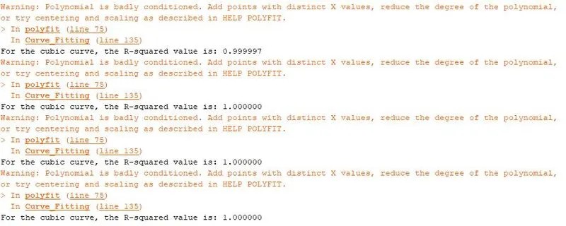
3. In error4, we can see there are centering and scaling warnings when a cubic polynomial is used (for every set) without scaling and centering (badly conditioned polynomial).
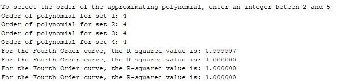
4. In correction1, we can see that after putting centering and scaling code, this warning message does not appear.

Conclusions:

1. How to make a curve fit perfectly?

• Remove the centering and scaling errors. Try using a higher-order polynomial with centering and scaling.

2. How to get the best fit?

• For the best fit, it is essential to split the data set and use the appropriate polynomial order for each set.

3. What could be done to improve the cubic fit?

• To improve a cubic fit, use centering and scaling and if possible, split the data and use a cubic fit for every set.

Removing Errors:

error1 = temp data was missing which was later added

error2 = polyfit output values were missing which was later added

error3 = disp command can take only one input argument, thus, multiple fprintf commands were used

error4 = badly conditioned polynomial, centering and scaling was used

correction1 = We can see that the warning (error4) for cubic polynomial is removed

Some additional graphs:

Splitwise method (all Quadratic curves)

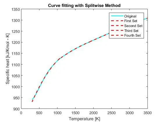
Splitwise method (all Cubic curves)

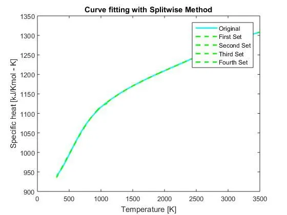
Splitwise method (all Fourth order curves)

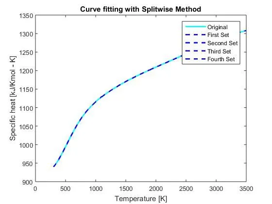
Splitwise method (all Fifth order curves)