Solving P-V Diagram of OTTO CYCLE using OCTAVE

AIM:

i)To create the P-V diagram for the otto cycle.

ii)To give the effeciency of otto cycle.

OTTO CYCLE:

The otto cycle is a thermodynamic cycle followed in gasoline engine.It consists of four process they are depicted as follows:

process 1-2: Isentropic compression

process 2-3: Isochoric heat addition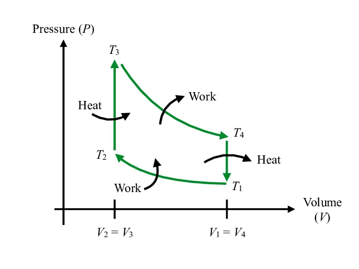

process 3-4:Isentropic expansion

process 4-1:Isochoric heat rejection

CODE SCRIPTED IN OCTAVE:

clear all
close all
clc

%definig inputs for state1 otto cycle %input p,t are in uppercase

%gamma variable
 Gamma = 1.4;
 
  P1 = 103125;
  T1 = 300;
  T3 = 2500;
  %engine parameters
  bore = 0.1;
  stroke = 0.047;
  connect_rod = 0.1;
  rc = 10;
  
  %volume definig for state1
  v_s = pi/4*bore^2*stroke;  %stroke volume
  v_c = v_s/(rc-1);  %clearance volume
    
  v1 = v_s+v_c; %total volume
   %state variable defining for  state 2
  
  constant_c = P1*v1^Gamma;
  
  %function piston_kinematics is called for compression curve
  
    V_compression =  piston_kinematics(bore, stroke, connect_rod, rc, 180,0);
    
    P_compression = constant_c./V_compression.^Gamma;
 
  
    v2 = v_c;
    p2 = constant_c/v2^Gamma; %PV^Gamma = constant_c,p1v1 = p2v2
    t2 = p2*v2*T1/(P1*v1);  
    
    
   %state variable defining for state 3
   v3 = v2;

   
   p3 = p2*T3/t2;
   
   constant_c = p3*v3^Gamma;
   
   %function piston_kinematics is called for expansion curve
  
    V_expansion =  piston_kinematics(bore, stroke, connect_rod, rc, 0,180);
    
    P_expansion = constant_c./V_expansion.^Gamma;
   
   %state variable defining for state 4
   v4 = v1;
   c = p3*v3^Gamma; %PV^Gamma = c
   
    p4 = c/v4^Gamma;
    t4 = p4*v4*T3/(p3*v3);  
   
   %plotting of points for the state conditions
   hold
   plot(v1,P1,'.','color','r')
   %Plotting of compression curve
   plot(V_compression,P_compression)
   plot(v2,p2,'.','color','r')
   %Plotting of Heat addition curve
   plot([v2 v3],[p2 p3],'color','b')
   plot(v3,p3,'.','color','r')
   %Plotting of expansion curve
   plot(V_expansion,P_expansion,'color','g')
   plot(v4,p4,'.','color','r')
   %Plotting of Heat rejection curve
   plot([v4 v1],[p4 P1],'color','b')
   
  %effeciency of otto cycle
   
   eff_otto = (1-(1/rc^(Gamma-1)))*100; %in terms of compression ratio
   
   s = T3-t2;
   q = t4-T1;
   
   ef_otto = (1-(q/s))*100; %in terms of state temperature  

#Here I use octave to write and present the code#

EXPLANATION OF THE CODE: We know that to start a code with clear all,close all,clc will be good so that it clears all the previous command.

DEFINING ENGINE PARAMETERS:

BORE(d)- It is the value of bore diameter of the cylinder where the piston reciprocates inside .The values obtained are made by assumption ,make sure to use reasonable value rather than choosing meaningless values.

STROKE(l)-It is the length of the cylinder along which the cylinder travels to and from top dead centre and bottom dead centre,the length of stroke will be smaller compared to bore dia for higher speed and oversquare engines.

CONNECT_ROD(L)-It is the length of connecting rod which connects the piston and the shaft which transmits the power to wheel.

rc-It is the compression ratio which is defined as the ratio of total volume and clearance volume i.e total volume is the sum of swept volume and clearance volume.

ASSUMED VALUES:

The following values are assumed to make the calculation easier which in real time is calculated experimentally.

p1(pressure at state1),t1(temperature at state1),t3(temperature at state1),Gamma(it is the air standard ratio of the otto engine).

FORMULA USED IN THE CODE:

Volume for swept:

`V=pi/4*d^2*l`

Adiabatic equation of the cycle:

`P*V^gamma = C`

Ideal gas equation:

`P*V=m*R*T`(Here mR is constant )

Volume trace equation:

The volume trace equation is used to follow the path that is followed by the cycle.Here R is the ratio of connecting rod length to the crank pin radius.

theta is the crank angle.

`V/V_c=1+1/2(r_c-1)[R+1-costheta-(R^2-sin^2theta)^(1/2)]`

Effeciency of otto cycle:

`eta = 1-1/(r_c)^(gamma-1)`

CALCULATING THE STATE VARIABLES(P,V):

The varibles for every state is calculated to represent the state.

we use the above adiabatic equation and ideal gas equation to calculate the values of variables at their respective state.

Since The variable(P,T) for the state 1 and temperature for state 3 is given as inputs,remaining variables can be calculated.

DEFINING FUNCTION:

Use of the function: The function is used to repeat a set of code only when it is called in the program,it can be called as many times as possible.Using function calling one can get the user input whenever it is called.

The function name and the filename should be same orelse it will give a error ,before calling a function you must define a function with appropriate syntax.Here i use piston_kinematics as the filename and function name

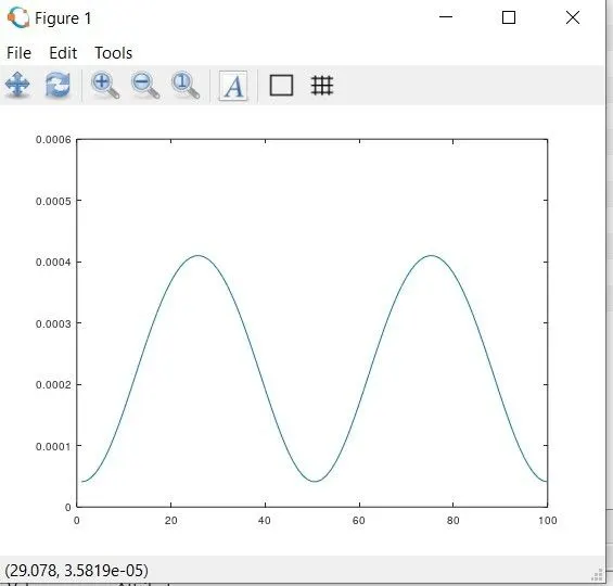
Here we use the volume trace equation for defining the equation.The volume trace eequation is splitted to three term for easy code definition.

CODE FOR DEFINING THE FUNCTION:

function [V] = piston_kinematics(bore,stroke,connect_rod,rc,start_crank,end_crank)
  
  %crank pin radius
  a = stroke/2;
  %ratio of connecting rod length to crank pin radius
  R = connect_rod/a;
  
  v_s = pi/4*bore^2*stroke;  
  v_c = v_s/(rc-1);
  
  %crank angle
  theta = linspace(start_crank,end_crank,100);
  
  %V/Vc=1+1/2(rc-1)[R+1-cos0-(R^2-sin^20)^1/2] %cos0 is cos theta
  
  term1= 0.5*(rc-1);
  
  term2= R+1-cosd(theta);
  
  term3= (R^2-sind(theta).^2).^0.5;
  
  V = (1+term1*(term2-term3)).*v_c;
  
 
  
end

`theta` is the crank angle,here we use array of values to the crank angle where the piston position changes continuously.linspace command is used to get the array of crank angle.

start_crank is the starting crank angle.

end_crank is the ending crank angle.

The function defined here is called in main program for plotting compression and expansion curve ,after calculating the compression and expansion volume ,we calculate the compression and expansion pressure.

The figure shows the plot of the function which is defined for two cycles spaced .

PLOTTING:

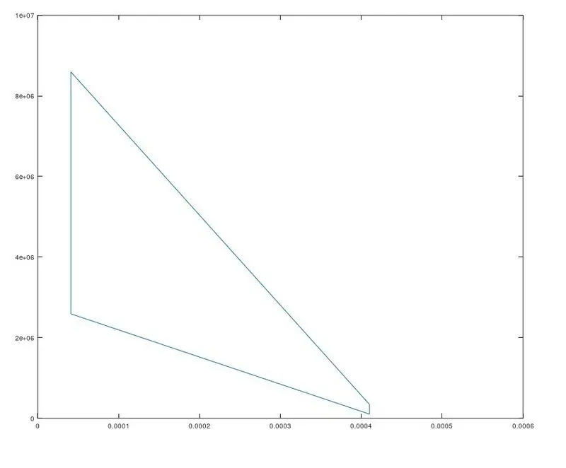
After calculating the values for the variable the next step we go is plotting the P-V diagram. PLOT command is used to draw the figure for P-V curve.Every point is plotted with volume at x-axis and pressure at y-axis.While using the following code it will gives a plot which follows a wrong path in the cycle

plot([v1 v2 v3 v4 v1],[P1 p2 p3 p4 p1]) the code will display the below figure

CONCLUSION:

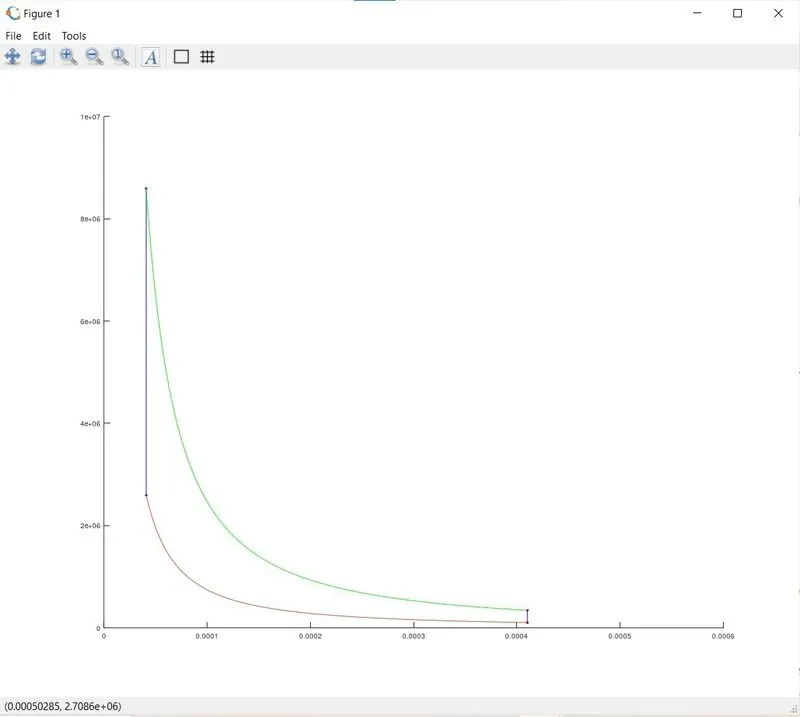
The output of the otto cycle is P-V diagram and the effeciency of otto cycle.

The following curve shows the figure for pressure-volume plot

The effeciency of otto cycle is depicted below:

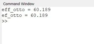The effeciency of otto cycle for the scripted code is 60.18%