Mixing efficiency

MIXING -T

AIM : To determine the Mixing -T simulation on different lengths and different inlet velocities in the ansys fluent

CASE -1

INTRODUCTION :

The T -cross section is most commonly used in many applications like power plants and other industry applications .In this T section the two fluids comes in to contact where as the hot fluid and the cold fluid .Now in this simulation process we are going to find out the temperature variations by using different lenghts and different velocities like keeping the hot fluid velocity constant and varying the cold fluid temperature .And by using the ansys fluent we are going to find out the temperature distribution and plots ,and we should see how the temperaure is varying on different velocities.

PRE-PROCESSING :

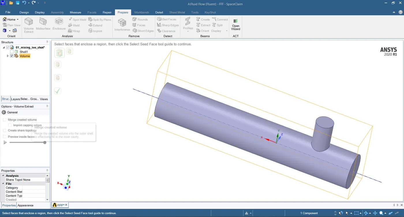
• click on the fluent and then click on the geometry and then open the spaceclaim and then import the geometry and then extract the parts that are not required in the simulation process ,as if we are not extracting the unnecessary parts it consumes some extra time during the process of solving so,it is good for extracting and for the completion of the process soon .
• And after extracting ,then supress the solid that which will be good for getting good results.
• And after that close the space claim .
• And then click on the MESH,in the mesh we are going to apply the mesh to the solid and then we are going to check the quality of the mesh .
• And in the mesh ,we are going to name the sections as per the requirement as hot fluid inlet ,cold fluid inlet and out let of the fluid and after assinging all the sections and then click on update in mesh.

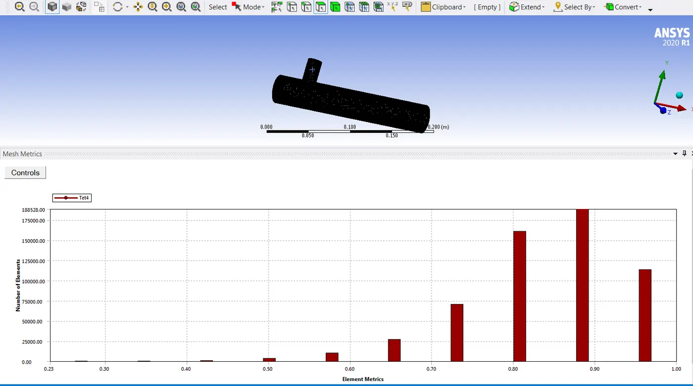
• Mesh quality properties
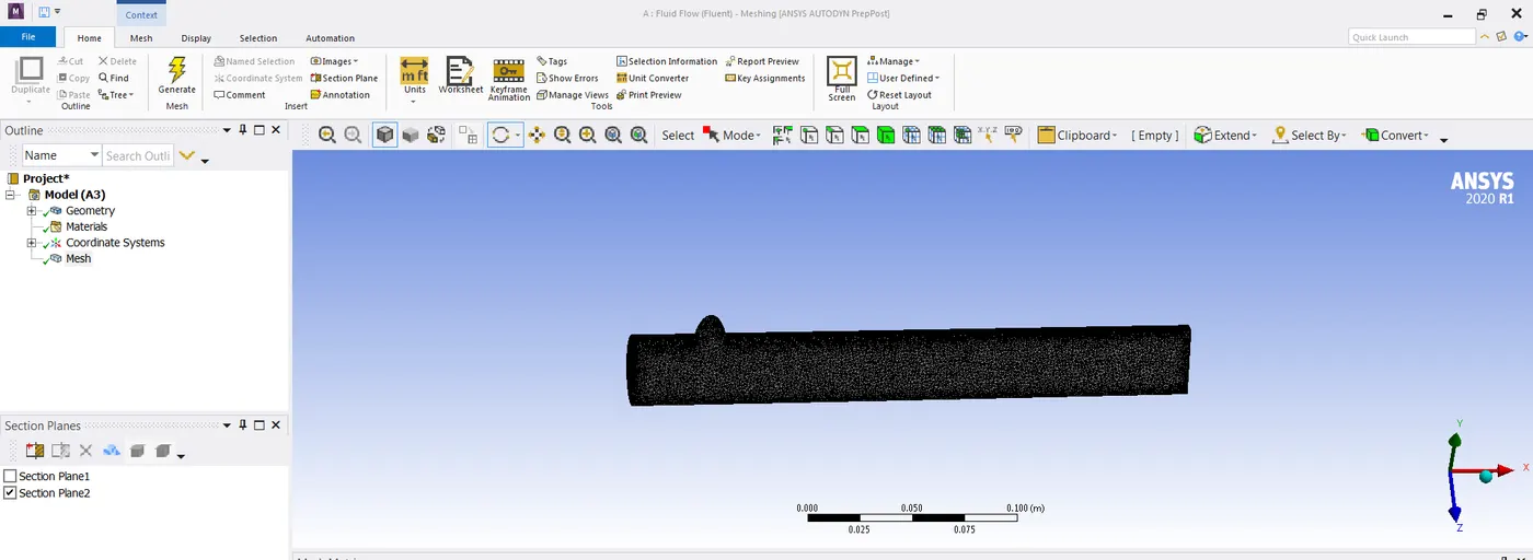
• cut sectional view

SOLVER :

• After meshing then go the solving process ,in this we will do all the steps that are required for the solution process.
• In this all the boundary conditions are given .
• short pipe -hot fluid inlet velocity -3m/s ,cold fluid inlet velocity 6m/s and 10m/s
• long pipe - hot fluid inlet velocity -3m/s , cold fluid inlet velocity 6m/s and 10m/s
• cold fluid temperature -283 k and hot fluid temperature 300k
• And after that add the materials and zones and select the plots and after all the process intiallize the process ,for better accuracy do the hybrid intialization .
• And run the calculation .

RESULTS :

• In this post processing process we can see all the results in the form of stream lines ,vectors and plots
• And by this we can see where the temperature is maximum and minimum and how it is varying by varying the velocities .

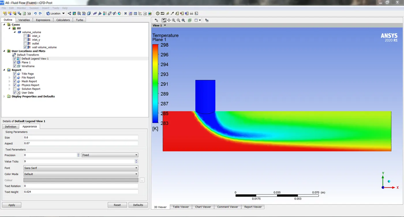
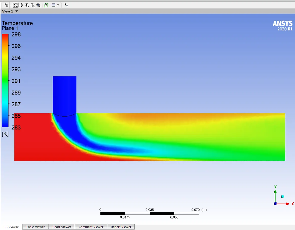
• short pipe hot fluid 3m/s-cold fluid 6m/s temperature variation

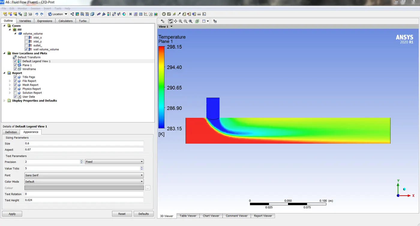
• hot fluid 3m/s-cold fluid10m/s -temperature variation

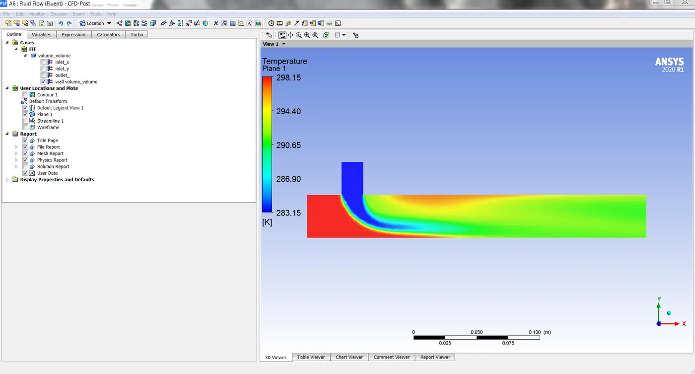
• long pipe hot fluid 3m/s -cold fluid 6m/s temeprature variation

• hotfluid 3m/s -cold fluid 10m/s temperature variation
• These are the results we get and above figures shows how the temperature is varying on varying the velocities and in the different lengths .

CONCLUSION:

• Coming to the conclusion ,from the above results we can conclude that by increasing the length of the pipe and by decreasing the velocity of the cold fluid we can get maximum heat tranfer between the fluids.
• As we see above figures ,long pipe with 3m/s and 6m/s there is contineous drop of the temperature and as coming to the long pipe 3m/s and 10m/s the temperature is droping but the transfered temperature not completely dispiating .
• so we can finally conclude that by increaing the length of the pipe and decreasing the cold fluid velocity we can get the better efficiency and can get better heat transfer.