MATLAB program to calculate drag force against a cyclist and obtain plots against varying velocities and drag co-efficient .

Matlab program to calculate drag force against a cyclist.

The task at our hands is to discuss and plot variation of drag force with varying velocities and varying drag coefficient for a rider riding a bicycle.

Let us use our existing knowledge to establish the equation we are working with and the parameters that we need to define to run our program and find the desired output.

First, let us discuss the eqaution of drag force:

Drag force = 0.5*density of medium*velocity^2*Frontal area*drag coefficient .......equation 1

Let us now define each parameters separately.

1) Density

Density of medium in our case will be the density of air.

Although variation in air density is possible with variation in altitude and temperature, we will assume the density of air to be the standard air density i.e. 1.225 kg/m^3 at 15 degrees celcius at sea level.

Dimensions of density is M^1*L^(-3)*T^0.

Note: This is a typical form of dimensional notation to specify the unit of the parameter in discussion. We will define all units in this dimensional notation to be flexible with all systems of measurement. "M" here stands for mass, "L" stands for lenght and "T" denotes time. There are only a few fundamental dimensional notation which one should know as all other units can be very easily expressed using these notations and a combination of their powers. For this project, the dimensioms M, L and T are sufficient to define all units.

For my program, I have used the variable name "rho" to define denity of air.

2) Velocity

We need to plot the graph for variation of drag force with variation in velocity.

I have considered that my analysis will be limited to the bicycle going as slow as 5 km/h to as fast as 35 km/h. Converting these values to the S.I. unit, we wil attempt to plot the values of velocity between 1.4 m/s to 8.5 m/s.

Dimension of velocity M^0*L^1*T^(-1)

For my program, I have used the variable name "velocity" to define velocity of rider riding the bicycle.

3) Frontal Area

Frontal area is the projection of the bicylce along with the rider when observed from a front view, i.e. facing the rider.

I have assumed the frontal area to be 0.36 m^2 as actual calculation is very subjective.

Dimension of area is M^0*L^2*T^0.

For my program, I have used the variable name "area" to define frontal area.

4) Drag Force

Drag force is the resistance expereinced by a body moving through a fluid due to the viscous property of the fluid. The factors which infleunce the drag force has already been mentioned in equation 1 above.

The dimension of drag force in M^1*L^1*T^(-2) or in S.I. units kgm/s^2 which is the unit in which we expect our output.

For my program, I have used the variable name "drag_force" to define drag force expreinced by the rider.

5) Drag Coefficient

Drag effecient is a empirically determined value on which the drag force is dependent. It is important to note that drag force is not a proportionality constant like gravitational constant. In fact, drag coeffcient depends on a number of factors like frontal are shape or form, smoothness of the fluid solid interface, Reynold's number and Mach number. For this program, I have used a velocity range in which we can assume Reynold's number and Mach number to have negligilble effect on change in drag coefficient. We will only consider change in frontal shape as our basis for change in drag coefficient.

Before finding out the values for drag coeffcient, let us first find out it's dimension.

From equation 1,

Drag coefficient=Drag force/(0.5*density of medium*velocity^2*Frontal area*) ....equation 2

Let us analyse it dimensionally

Unit of Drag coefficient = (M^1*L^1*T^(-2))/{(M^1*L^(-3)*T^0)*[(M^0*L^1*T^(-1))^2]*(M^0*L^2*T^0)} ......equation 3

From equation 3 we can see that Drag coefficient is a dimension less factor.

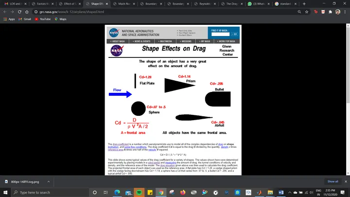
Now, here is an snapshot for variation of drag coefficient with variation of frontal shape or from ever though the frontal area is same.

IMG 1: Source: https://www.grc.nasa.gov/www/k-12/airplane/shaped.html

From the image above we can observe that, highest drag coefficient is for a flat plate i.e. 1.28 and the lowest is for air foil i.e. 0.45. All other values of drag coeffcient lies between these two limits. In my program I will be using this knowledge to define drag coeffcient matrix.

Since we have discussed the underlying theory behind our program, let us now understand how to code it in MATLAB

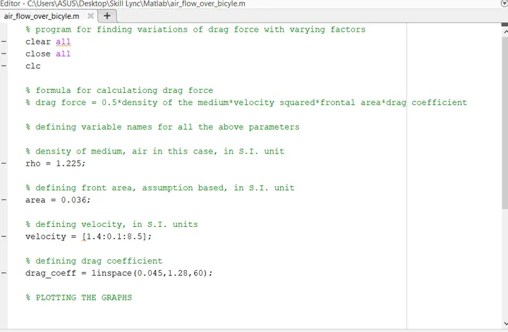
1) Let us first understand the variable declaration.

From the snapshot below

IMG 2

Density of air and frontal area are treated as constant in this program and I have assigned values to them in the following commands:

rho = 1.225;

area = 0.036;

For defining velocity, as discussed already, i have taken limits of 1.4 and 8.5. I have used colon operator to create small steps between each value of velocity through the code:

velocity = [1.4:0.1:8.5];

By doing so, i am able to genrate many points so that my curve will appear smooth.

Similarly for defining drag coeffcient, I have used linspace command. The limts that is to be used has already been defined, Through linspace I can instruct MATLAB to generate desired number of equidistant points between two limits. In this case I have instructed MATLAB to generate 60 equidistant points between 0.045 and 1.28 inclusive of the limits. Higher the number of points, smoother will be the curve generated.

So, now since we have defined all our parameters through variables, let us move forward to calculate drag force and plot our desired graph.

IMG 3

Code in MATLAB:

% program for finding variations of drag force with varying factors
clear all
close all
clc

% formula for calculationg drag force
% drag force = 0.5*density of the medium*velocity squared*frontal area*drag coefficient

% defining variable names for all the above parameters

% density of medium, air in this case, in S.I. unit
rho = 1.225;

% defining front area, assumption based, in S.I. unit
area = 0.036;

% defining velocity, in S.I. units
velocity = [1.4:0.01:8.5];

% defining drag coefficient
drag_coeff = linspace(0.045,1.28,60);

% PLOTTING THE GRAPHS


% step 1: variation with speed

drag_force = rho*velocity.^2*area*drag_coeff(30)*0.5;
plot(velocity, drag_force,'color','b')
xlabel('VELOCITY')
ylabel('DRAG FORCE')
grid on


% step 2: variation with drag coeffcient

% drag_force = rho*velocity(30)^2*area*drag_coeff*0.5;
% plot(drag_coeff, drag_force,'color','r')
% ylabel('DRAG COEFFICIENT')
% xlabel('DRAG FORCE')
% grid on

Code 1

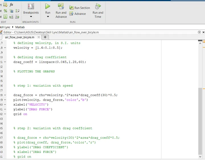
The codes from line 28 till line 32 is the code for plotting drag force vs velocity graph.

Notice that for squaring velocity matrix, I have used dot (.) operator before squaring it so that I can instruct MATLAB to perform dot product on velocity matrix which will be fufiling my requirement for using square of velocity in my drag force calculation.

Also, note that since I have already defined my drag force matrix, I can simply call a value from it and use in as a constant for my equation(i.e. drag_coeff(30), which is the 30th value of the matrix drag_coeff). By doing so, I am able to avoid unecessarily declaring variables and making the programm clumsy.

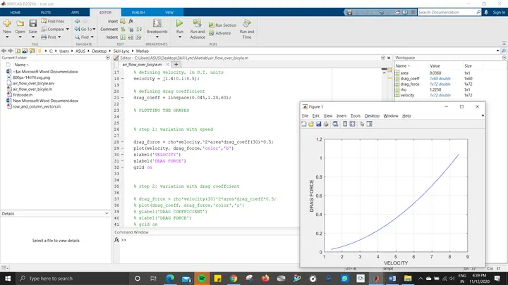
Now, from equation 1 and command in line 28, I expect my graph to be a quadratic equation of the form y=mx^2.

In line 29, I have used the plot command and chose to plot my grpah in blue colur. Subsequently, I have also define my x and y axis through x-label and y-lablel commands. I have also enabeld the grid through command in line 32.

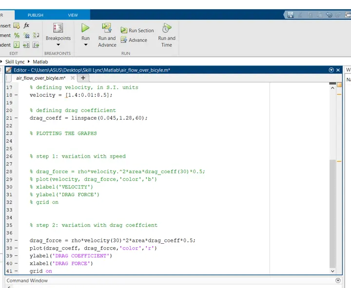
Also note that I have already done the coding for ploting drag coeffcient vs drag force graph in lines 37 through 41, but I have turned them into comments so that they don't get executed.

Now let us check our plot.

IMG 4

Our plot is much in accordance to our prediction.

However, this may not always be the case. Let me demonstrate by an example.

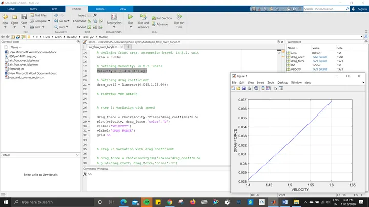
At, this point I would like to redefine my velocity matrix as velocity = [1.4:0.01:1.6]; and rerun the code.

Let us check our plot again.

IMG 5

Notice now that my graph is almost like a straight line. However, this plot is both matematically and practically accurate. The simple explanation for this is the fact that when are decreasing the limits, we are essentially finding the differential of the curve at a point, which we know from our high school mathematics is a straight line with a certain slope. The purpose of discussing this observation was to emphasize the fact that sometimes visual representation may be counterintuitive even though they are mathematically and practically true.

Now let us move to our second plot. I have already uncommented lines 37 through 41 and commented line 28 through 32 to avoid any error. Also i have stored the values of velocity to original values.

IMG 6

Code in MATLAB

% program for finding variations of drag force with varying factors
clear all
close all
clc

% formula for calculationg drag force
% drag force = 0.5*density of the medium*velocity squared*frontal area*drag coefficient

% defining variable names for all the above parameters

% density of medium, air in this case, in S.I. unit
rho = 1.225;

% defining front area, assumption based, in S.I. unit
area = 0.036;

% defining velocity, in S.I. units
velocity = [1.4:0.01:8.5];

% defining drag coefficient
drag_coeff = linspace(0.045,1.28,60);

% PLOTTING THE GRAPHS


% step 1: variation with speed

% drag_force = rho*velocity.^2*area*drag_coeff(30)*0.5;
% plot(velocity, drag_force,'color','b')
% xlabel('VELOCITY')
% ylabel('DRAG FORCE')
% grid on


% step 2: variation with drag coeffcient

drag_force = rho*velocity(30)^2*area*drag_coeff*0.5;
plot(drag_coeff, drag_force,'color','r')
ylabel('DRAG COEFFICIENT')
xlabel('DRAG FORCE')
grid on

Code:2

Once again I have defined drag force as I had done for the previous plot, selecting a specific value from velocity matrix and using the entire drag coeffcient matrix. This time I have chosen to colour my plot line in red.

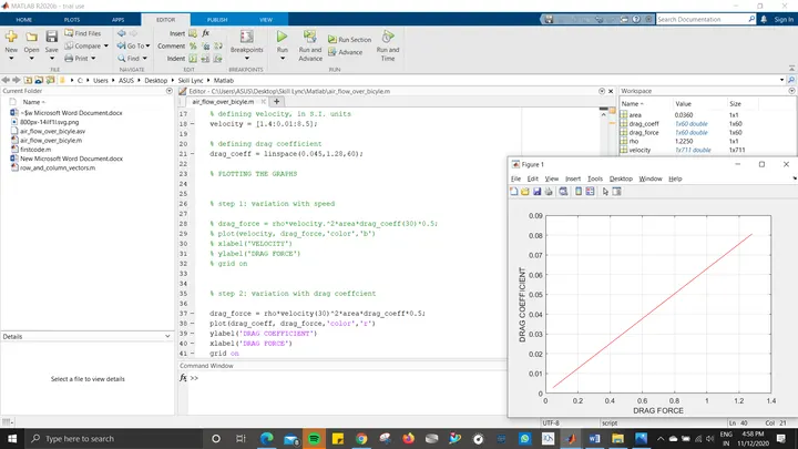
The command in line 37 is an equation of the form y=m*x which is the equation of a straight line.
Now let us check our predcition.

IMG 7

So the plot obtained is very accurate to our prediction.

Hence, we have discussed various parameters governing drag force on a cyclist and were successful in plotting the velocity vs Drag force graph and Drag coefficient vs Drag force graph and the results were in accordance with our prediciton.