Week 3 - Solving second order ODEs

Solving 2nd Order ODE in MATLAB and simulating pendulum motion

• Introduction

Many factors in an equation are derivative of a function(s). A function may depend on more that one parameter. As a result, we need to choose between the Partial differential equation(PDE) and the Ordinary differential equation(ODE) based on the problem. ODE is an equation in the derivative of only one variable while PDE deals with factors depending on more than one parameter. For example, consider the equation of motion s = u*t + (1/2)*a*t^2 ...eq_1. The parameter "u" i.e. initial velocity is the differential of displacement w.r.t. time. Similarly, "a" denotes the 2nd derivative of displacement w.r.t. time. So equation 1 is a 2nd Order ODE w.r.t time. Examples of PDE is stream equation in 2-D or 3-D since the flow pattern will depend on parameters acting in all cartesian directions i.e. along x.y and z axes.

• Ordinary differential equation

The focus of this report will be on ODE. We have learnt that PDE can be solved by using formulae or by numeric methods. When we use the formula to solve an ODE, an accurate solution is obtained but it is difficult to achieve through coding. Numeric methods are preferred in computationally solving an ODE. Matlab also contains many ODE solver functions viz. ode23, ode45, ode15i and they can be used depending upon the problem.

ODE describing the motion of a pendulum or a spring-mass system is an ODE of order 2 and can be solved in Matlab using the function ode45.

• Mathematical modelling

The equation of a spring-mass system of a simple pendulum appears as following:

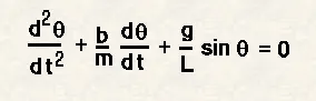
Image:1

The term "Theta" in image 1 represents displacement in the case of a spring-mass system and angular displacement in the case of a simple pendulum.

The objective of this code is to simulate simple pendulum motion using the equation in image 1.

W.r.t. image 1

theta = angular displacement

b = damping co-efficient = 0.05 kg/s.

m = mass of the pendulum ball = 1 kg,

g = accelertaion due to gravity = 9.81 m/s2.

L(or l) = length of pendulum string = 1 metre

t = time

Matlab can solve ODE in 2nd order by converting it to a system of 1st order ODE.

Let,

theta = theta1

theta2 = d(theta1)/dt ...eq_2 - d in the equation denotes derivative

So, image 1 becomes

d(theta2)/dt = -(b/m)*theta2 - (g/l)*sin(theta1) ...eq_3

So, equations 2 and 3 are two 1st order ODE represnting the equation in image 1.

The solution matrix therefore becomes theta = [theta1;theta2] ...eq_4.

• Matlab Code

1.	clear all
2.	close all
3.	clc

4.	%Defining various fixed parameters
5.	%Fixed parameters are provided in the problem statement
6.	b=0.05; %Damping Coefficient S.I. units
7.	g=9.81; %Acceleration due to gravity S.I. units
8.	l=1; %Length of the pendulum string S.I. units
9.	m=1; %Mass of the pendulum ball at the end of pendulum string in S.I. units

10.	%{ 
11.	Next step includes defining the initial value: A column array containing two
12.	elements namely "Initial Displacement" and "Initial Angular Velocity"
13.	%}
14.	theta_t_0 = [0;3]; %Provided in the problem statement in S.I.units

15.	%Next step is defining time span within which various plots will be
16.	%obtained 
17.	time_span = linspace(0,20,1000);%thousand instances of time between 0-20 will be created 


18.	%Next step is solving the system of linear ODE(s) 
19.	[t,result] = ode45(@(t,theta) ode_func(t,theta,b,g,l,m),time_span,theta_t_0);

20.	hold on
21.	grid on
22.	plot(t,result(:,1))
23.	plot(t,result(:,2),'LineStyle','--')
24.	ylabel('plot')
25.	xlabel('time')
26.	legend('Angular Displacement','Angular Velocity');
27.	pause(3);
28.	text(10,-2.7,'Wait for the Animation');
29.	pause(4)
30.	hold off
31.	clf



32.	%Code for animation
33.	t1 = l;
34.	t2 = result(:,1);
35.	swing = l*sin(t2);
36.	leg = 0 - t1*cos(t2);



37.	frame=1
38.	for i=1:1:length(swing)

39.	grid on
40.	hold on
41.	x = [0 swing(i)]
42.	y = [0 leg(i)]
43.	axis([-1 1 -1.2 0.2]);
44.	handle = line(x,y);
45.	handle.Color = '#A2142F';
46.	handle.LineWidth = 3;
47.	plot(swing,leg,'LineWidth',0.0002,'LineStyle',':');
48.	plot(0,0,'.','MarkerSize',70,'Color','#0072BD');
49.	plot(0,0,'.','MarkerSize',35,'Color','#000000');
50.	plot(swing(i),leg(i),'.','MarkerSize',100);
51.	% plot(0,0,swing(i),leg(i),'LineWidth',20);

52.	hold off
53.	Mov_frame(frame) = getframe(gcf);
	 frame = frame+1
54.	clf

55.	%for checking consistency of the length of pendulum string
56.	lengthofstring(i) = sqrt(swing(i)^2 + leg(i)^2);
57.	end

58.	movie(Mov_frame);
59.	video = VideoWriter('ODE solver');
60.	open(video)
61.	writeVideo(video,Mov_frame)
62.	close(video)

63.	%Furthermore, we need to define our ODE
64.	function[dtheta_dt]=ode_func(t,theta,b,g,l,m)
65.	theta1 = theta(1)
66.	theta2 = theta(2)
67.	dtheta1_dt = theta2;
68.	dtheta2_dt = (-b/m)*theta2 - (g/l)*sin(theta1);
69.	dtheta_dt = [dtheta1_dt;dtheta2_dt];
70.	end

Code:1

In line 14, initial conditions have been defined. The quantity theta2 denotes angular velocity, and theta1 denotes angular displacement. The formulation of a set of 1st order ODE, as defined in the previous section, is achieved through a user define function ode_func and the same is described in line numbers 64 through 70 in the code as shown in the code snippet above.

In line 14, 20 second time is divided into 1000 part and each value of the array time_span will be used to find a solution to the ODE.

Line 14 describes the use of ode45 to obtain a solution set. The syntax of ode45 can be found in Matlab help. The solution of ode45 is stored in the array [t,result]. The various t contains 1000 instances of time obtained through code in line 17. The variable result is an array of two columns and it contains the values of theta1 and theta2 for each value of the array t. The result variable is hence the solution set.

The next aim is to obtain the plots and make an animation out of the plots.

• Plot 1

The first plot will help to visualise how theta changes with time. Refer to line 20 through 31. The plot command in line 22 will plot values of theta1(angular displacement) w.r.t. each element in array t(time). Similarly, line 23 will plot values of theta2(angular velocity) w.r.t. each element in array t(time). Legends, labels, etc may be added as per requirement. The pause command has also been added as there is a trailing plot command. Without pause command, this plot will be difficult to observe. Notice the clf in line 31. The clf command is used to clear the plot screen. It is instrumental in obtaining the animation in this program. The output is as following:

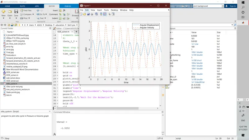
Image 2:

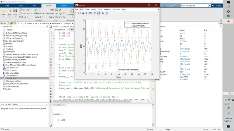
Image 3:

For making the plots interesting, I have added a text on the plot "Wait for the Animation" as the next plot(s) will be used to form the animation video. Notice the plot for theta2. Through code in line 23, I have altered the plotline style, making it easy to visualise the plot.

As clearly observable, the wave-like plots are decreasing over the subsequent cycles. It's an assurance that the motion is indeed a damped motion and the wave-like plot ensures that it's an oscillating motion. Hence we can conclude that the plot obtained is the motion of an oscillating pendulum.

In the next section, plots will be obtained to make an animation.

• Plot 2

To obtain the plot for animation, understanding the geometry of the pendulum in motion will be important. Observe the image below:

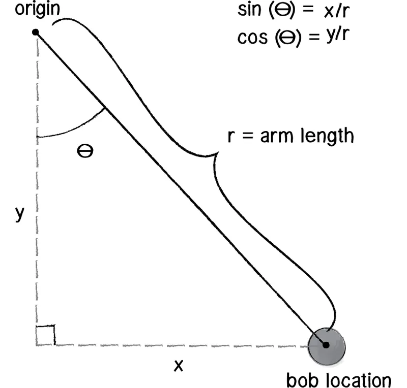
Image 4:

The centre of the pendulum ball(bob as per the image) can be defined using elementary trigonometry. The hinge(origin as per the diagram) can be assumed at the cartesian point (0,0).

The position of the ball is given by:

x-coordinate: l*sin(theta) (Code line 35: variable name: swing)

y-coordinate: 0 - l*cos(theta) (Code line 35: variable name: leg)

Different values of theta have already been calculated and stored in the 1st column of the result matrix.

For creating the thread on the pendulum, I have used the line function(Refer code line 44: variable name handle). Properties of the line segment thus created can be altered based on the requirements.

Through the for loop in line 38 of the code, I have ensured that a plot is obtained for all values of theta1.

the plot commands in line 48,49 and line 50 of the code are for points at the hinge and the pendulum ball respectively.

The plot in line 47 displays an arc corresponding to the motion of the pendulum ball. This plot will be useful to visualise the decay of the pendulum oscillation.

Notice the codes in line 37, 53 and 58 through 62. These codes are useful to create the animation. The objective is to record each plot and combine them to form a video.

The output of the second plot are following:

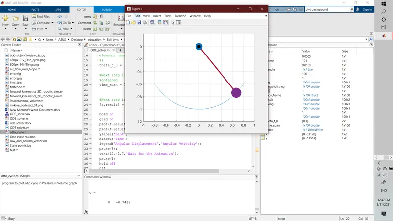
Image 5:

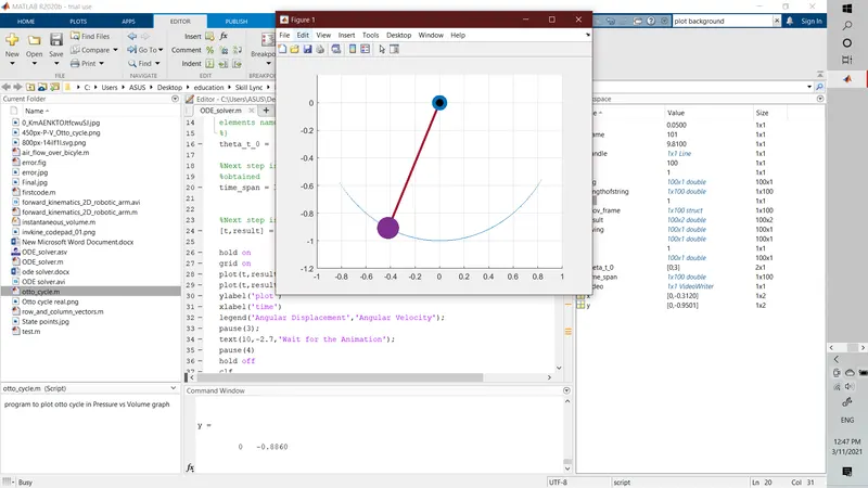
Image 6:

Matlab will plot 1000 plots one after another and it will appear almost like a video. After the execution of the code, the video file will be saved in the pre-defined directory.

Youtube link for video: https://www.youtube.com/watch?v=Kzg9GODRHes

• Errors and debugging

It is important to confirm the unit of theta i.e. degrees or radians as the trigonometric functions in Matlab are different for different units. To keep a check, I have put a checking condition at code line 56. After the program completes its execution, all values of the array variable lengthofstring(which find the distance between the hinge and the centre of the pendulum ball) must be equal to the length of the string. Observe the image below.

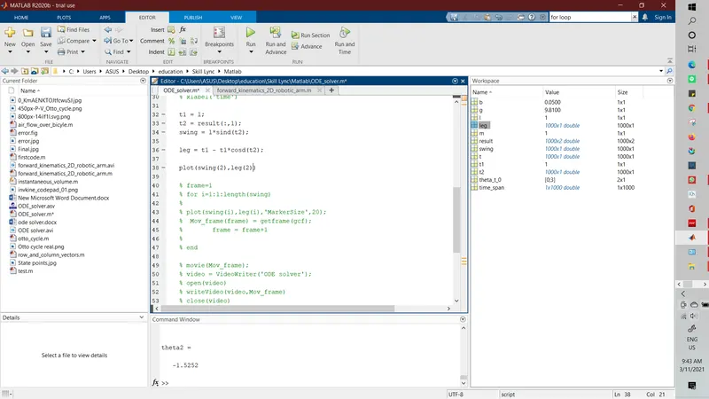
Image 7:

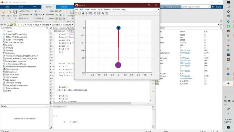
Image 8: Notice how the arc below has disappeared on plotting with cosd and sind functions.

Notice the code line 31 with clf command. All the plots within the for loop, as described in the previous section, need to be obtained on a single plot. Hence, we have to use the hold command. However, doing so will combine all the other plots as well and animation will fail. The clf command at the end of the loop ensures that the plot screen is cleared at the end of the loop. Observe the following image.

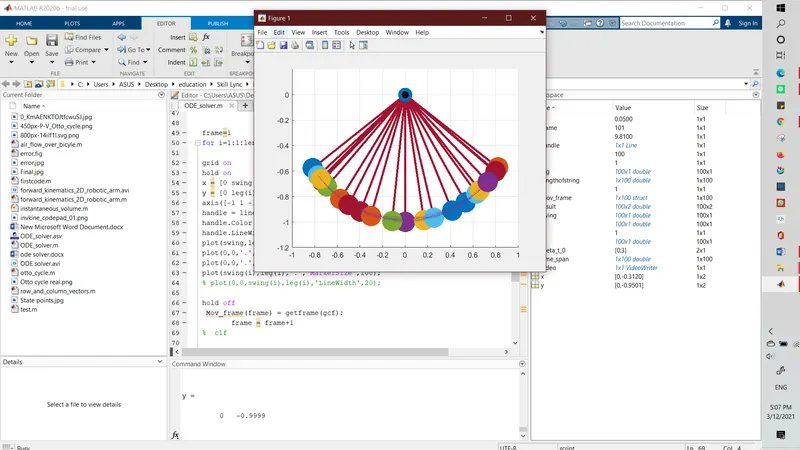
Image 9:

Thirdly, the plot screen should not be minimised or maximised. Doing so will result in an error and Matlab cannot form the video due to differences in sizes of the plot screen. See the images below.

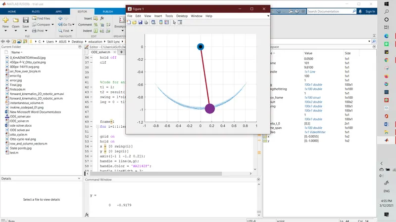
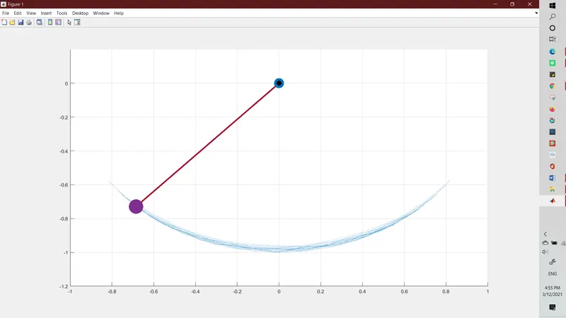
Image 10 & 11:

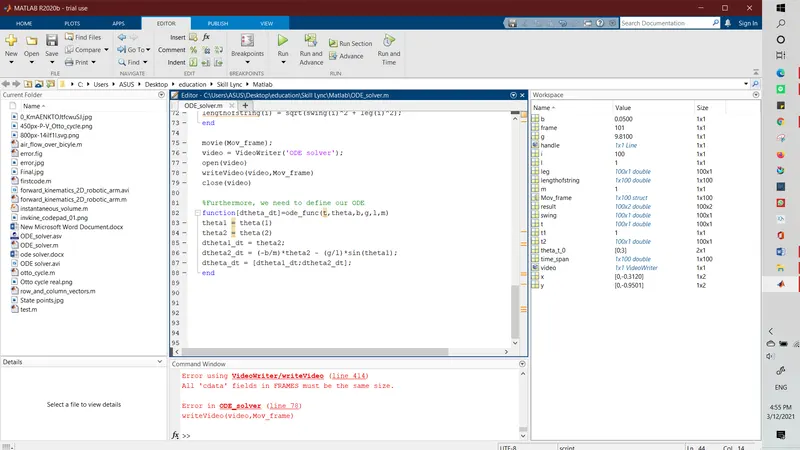
Image 12:

• Conclusion

This project is a good starting point to comprehend a vector-based image or video. In addition, the syntaxes of Matlab ODE solvers are very useful albeit difficult to comprehend.