MATLAB code that can solve an Otto cycle and make plots for it in the PV diagram while calculating and displaying the thermal efficiency of the engine. -Tanmay Dash
Challenge: Write code that can solve an otto cycle and make plots for it.
- Plot to be made in PV diagram
- Thermal efficiency of the engine is needed to be calculated and displayed.
Section1: Introduction
Otto cycle is an air standard cycle, i.e. the working agent is considered to be air and hence ideal gas equation and thermal properties of air can be used to calculate various state points and processes.
Otton cycle is an ideal cycle which is the closest estimation to the thermodynamic processes in a petrol engine. Otto cycle consists of two constant volume or isochoric processes and two isentropic or constant entropy or adiabatic processes. Heat addition and rejection happens during isochoric processes in the cycle.
A thermodynamic cycle is a cyclic process in thermodynamics when the system returns to initial state point after several processes.
Following is the illustration of otto cycle in a Pressure vs Volume diagram:
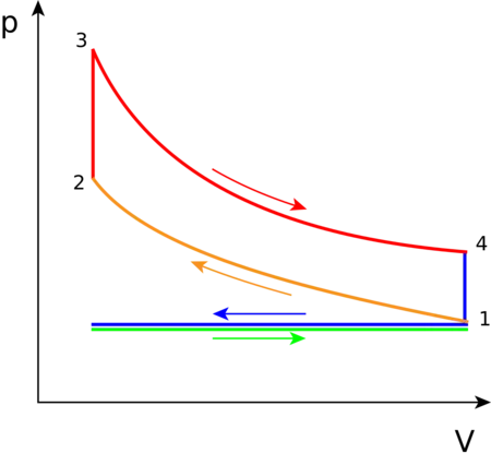
Figure: 1) Green and blue line are the compensation for air intake in an actual cycle, which is not a part of the otto cycle
To contrast the approximations made in the ideal cycle as compared to real petrol cycle, the following is an illustration of the otto cycle in a petrol engine.
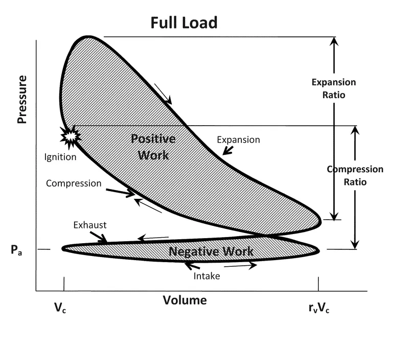
Figure: 2) Actual petrol cycle
Section2: Underlying thermodynamic phenomena
Otto cycle has 4 distinct state point which is related by thermodynamic processes. At, this point it would be prudent to point out that cyclicity of the process can only be ensured if all processes are assumed to be reversible.
With reference to figure1, four state points can be identified as state point 1, state point 2, state point 3 and state point 4.
The process from state 1 to state 2 is an isenthalpic or adiabatic compression. At state 2, the working agent is ignited. So from state 2 to state 3, the cycle gains energy in form of heat which is produced due to conversion of chemical energy in the air-fuel mixture into thermal energy. Since this process happens almost instantaneously, i.e. at the top dead centre of the engine, the volume of the mix remains almost constant. So process 2 to 3 is termed as isochoric or constant volume heat addition process. From state point 3 till state point 4, the increase in pressure due to sudden addition of heat pushes the piston towards the bottom dead centre and the mechanical work is produced in the process. Hence process 3-4 is also called a power stroke or expansion stroke. The engine in an ideal otto cycle is assumed to have no heat loss to the environment. So similar to process 1-2, process 3-4 is also adiabatic. Now, at state 4, it is assumed that the system purges all the burnt working agent instantaneously when the piston is at bottom dead centre, and along with the residual thermal energy in the working substance is also lost to the environment. Hence, process 1-4 is described as the isochoric heat rejection process.
To summarise
Process 1-2: Adiabatic compression
Volume decreases
Pressure increases
Temperature increases
Process 2-3: Isochoric heat addition
Volume remains unchanged
Pressure increases
Temperature increases
Process 3-4: Adiabatic expansion
Volume increases
Pressure decreases
Temperature decreases
Process 4-1: Isochoric heat rejection
Volume remains unchanged
Pressure decreases
Temperature decreases
Section3: Mathematical modelling
Now that we are aware of the underlying thermodynamic processes, the task at hand is to calculate the state points, so that an appropriate graph may be plotted.
Terminologies
v1: volume at state point 1
v2: volume at state point 2
v3: volume at state point 3
v4: volume at state point 4
p1: pressure at state point 1
p2: pressure at state point 2
p2: pressure at state point 3
p4: pressure at state point 4
t1: temperature at state point 1
t2: temperature at state point 2
t3: temperature at state point 3
t4: temperature at state point 4
p1 = atmospheric pressure at STP: i.e. 101325 pascal
t1 = assuming the working is heated to 80-degree Celcius at entry, is 353K
v1 = summation of swept volume and clearance volume ....equation1
vswept = swept volume, is the volume of working agent compressed by movement of piston from bottom dead centre to top dead centre
vclearance = clearance volume, is the volume of fully compressed working agent
For calculating v1, vswept and vclearance, we have to take help of engine kinematics
Consider the following terminologies
bore: piston diameter
stroke: maximum length, that the piston can travel in one direction
cr: compression ratio i.e. ratio of net cylinder volume to clearance volume
length_cr: length of connecting rod
crankpin_rad = stroke/2: crankpin radius, used for engine kinematic calculation for plotting graph
R : length_cr/crankpin_rad;
gamma: isentropic process index for air
Now we can have following calculations:
vswept = pi*(bore^2)*stroke/4 ....equation2
vclearance = vswept/(cr-1) ....equation3
v1 can be calculated from equation1
At this point we know p1,v1 and t1
For calculating state point 2:
Process 1-2 is adiabatic process and the equation pv^gamma=constant (.....equation4) can be used to compute pressure at point 2.
p2 = p1*cr^gamma ........equation6
Replacing pressure with tempearture in equation4 using ideal gas equation pv=nrt(p: pressure, v:volume,n:moles of gas, r:universal gas constant, t:temperature.........equation5), t2 can be calculated as:
t2 = t1*cr^(gamma-1) .......equation7
v2=vclearance
For calculating state point 3:
The 3rd state point encounters maximum heat and pressure and is limited by material constraints. Usually, the metallurgic property of engine material changes at very high temperature and may be considered as a limitation to fix the temperature at state 3.
t3 = 2300K, based on material constraints
p3 = t3*p2/t2, from equation5 since volume is constant .......equation8
v3=v2, process 2-3 is constant volume process
For calculating state point4
p4 = p3/(cr^gamma), from equation4 .......equation9
t4 = t3/(cr^(gamma-1)), from equation5 .....equation10
v4=v1, since process 4 to 1 is again an ischoric process.
Now, that the calculations of all points have been established, the graph needs to be plotted.
However, the graph of the otto cycle possesses another challenge as process 1-2 and 3-4 are not straight lines, but follow equation 4. To find the plot the graph of adiabatic processes, engine kinematics needs to be used to find state variables volume and pressure in relation to crank angle.
instantaneous_volume/vclearance =
1+(1/2)(compression ratio−1)(𝑅+1−𝑐𝑜s(theta)-(R^2−𝑠𝑖𝑛(theta)^2)^0.5) .....equation11
R = connecting rod length/crank radius
Once the instantaneous volume is calculated from equation11, instantaneous pressure can be calculated using equation4.
Further elucidation will be provided through the Matlab code.
Section4: Coding in MATLAB
The following snippet shows the code that has been written in MATLAB to obtain the desired plot.
%program to plot otto cycle in Pressure vs Volume graph
clear all
close all
clc

%Step 1 : finding state variables for 4 points

% Engine kinematic paramters:
% inputs: bore of piston, stroke of piston, clearance ratio and lenght of connecting rod.

bore = 0.085; %bore or piston diameter of cylinder in m
stroke = 0.095;%length of stroke in m
cr = 10;%compression ratio i.e. ratio of cylinder volume to clearance volume
length_cr = 0.16; %lengthof connecting rod
crankpin_rad = stroke/2; %crank pin radius, used for engine kinematic calculation
R = length_cr/crankpin_rad;
gamma = 1.4; %isentropic process index for air
vswept = pi*(bore^2)*stroke/4; %swept volume from engine design paramters
vclearance = vswept/(cr-1); %obatined from compression ratio defintion


% Variables state 1
p1 = 101325; %in Pascal, pressure exterted by air at S.T.P.
t1 = 353; %in Kelvin assuming air at intake is heated to 80 degree celcius
v1 = vswept + vclearance; %total volume of cylinder is the summation of clearance volume and swept volume


% Variables state 2
v2 = vclearance;
p2 = p1*cr^gamma;%from isentropic process equation P*V^gamma = constant
t2 = t1*cr^(gamma-1); %from isentropic process equation and ideal gas equation P*V = n*R*T

% Variables state 3
t3 = 2300; %highest temp is a material constraint and hence defined before design;
v3 = v2; %process 2-3 is isochoric process
p3 = t3*p2/t2; %from ideal gas equation

% Variables state 4
v4 = v1; %process 4-1 is again isochoric process
p4 = p3/(cr^gamma); %from isentropic process equation
t4 = t3/(cr^(gamma-1)); %from isentropic process equation and ideal gas equation


const1 = p1*(v1^gamma);
const2 = p3*(v3^gamma);

volume_proc_1_2 = instantaneous_volume(bore,stroke,length_cr,cr,180,0);
pressure_proc_1_2 = const1./volume_proc_1_2.^gamma;
volume_proc_3_4 = instantaneous_volume(bore,stroke,length_cr,cr,0,180);
pressure_proc_3_4 = const2./volume_proc_3_4.^gamma;

%thermal efficiency claculation

eff_ther = (1-cr^(1-gamma))*100;

hold on
plot(v1,p1,'o','color','r')
plot(v2,p2,'o','color','r')
plot(v3,p3,'o','color','r')
plot(v4,p4,'o','color','r')
plot(volume_proc_1_2,pressure_proc_1_2,'color','b');
plot([v2 v3],[p2 p3],'color','b');
plot(volume_proc_3_4,pressure_proc_3_4,'color','b');
plot([v4 v1],[p4 p1],'color','b');
str = {'Thermal efficiency of given otto cycle (in percentage)is: ',eff_ther};
text(v3+v3,p3,str)
xlabel('Volume(m^3)')
ylabel('Pressure(Pascal)')
grid on
Code1
All the details provided in the mathematical modelling has been coded by providing the required input.
Various engine kinematic parameters have been defined arbitrarily.
However, we can see a function named "instantaneous_volume", which has not been addressed as of yet.
In reference to the code below:
function [v] = instantaneous_volume(bore,stroke,length_cr,cr,start_angle,end_angle)
%instantaneous volume/clearance volume =
% 1+(1/2)(compression ratio−1)(𝑅+1−𝑐𝑜s(theta)−(R^2−𝑠𝑖𝑛(theta)^2)^0.5)
%R = connecting rod length/crank radius
vswept = pi*(bore^2)*stroke/4;
vclearance = vswept/(cr-1);
crankpin_rad = stroke/2;
R =  length_cr/crankpin_rad;
theta = linspace(start_angle,end_angle,180);

term1 = cr - 1;
term2 = R + 1 - cosd(theta);
term3 = (R^2 - sind(theta).^2).^0.5;
term4 = 1 + 0.5*term1*(term2 - term3);
v = vclearance*term4;
end
Code2
A function has been defined to calculate the instantaneous volume of the working agent in the petrol engine, using equation11.
We have used linspace command to create and an array of angular positions of the piston, which can be used further to produce an array of instantaneous volumes.
Notice that equation11 has been fragmented into term1, term2, term3 and term4 to avoid calculation errors and maintain the aesthetic of the program.
In code1, the function "instantaneous_volume" has been, and required arguments have been passed to obtain an array of instantaneous volume.
The array, "volume_proc_1_2", stores various values for volume of the working agent at different angles of crankshaft starting from 180 to 0(Bottom dead centre to top dead centre).
Similarly, the array "volume_proc_3_4" stores various values for volume of the working agent at different angles of crankshaft starting from 0 to 180(Top dead centre to bottom dead centre).
Next, we need to find the instantaneous pressure values at various crank angles.
We can use equation4 to find instantaneous pressure arrays. For that, we have defined the constant using the already know state parameters at points 1 and 3. Note that the value of constant is different for process 1-2 as compared to 3-4 and using the same constants will produce a graph somewhat as shown below.
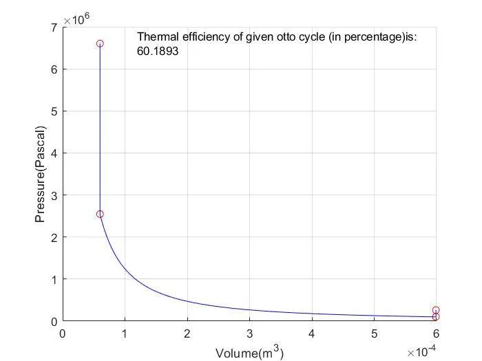
Figure3: Notice that due to using same constant, process line 3-4 has merged with process line1-2
So we have chosen two constant and defined as follows:
const1 = p1*(v1^gamma); ......equation12
const2 = p3*(v3^gamma); .......eqaution13
Using equations 12 and 13, and performing dot product with instantaneous volume matrices we get pressure matrices as following:
pressure_proc_1_2 = const1./volume_proc_1_2.^gamma; .....equation14
pressure_proc_3_4 = const2./volume_proc_3_4.^gamma; .....equation15
Now we have got all the points to plot the graph.
Starting with hold on command, to allow mutliple simultaneous plots, we first plot all state point as;
plot(v1,p1,'o','color','r')
plot(v2,p2,'o','color','r')
plot(v3,p3,'o','color','r')
plot(v4,p4,'o','color','r')
The third argument in plot command i.e. 'o' is the marker at the state point.
Now we need to plot process lines, using following commands:
plot([v2 v3],[p2 p3],'color','b');
plot([v4 v1],[p4 p1],'color','b');
Above command joins point 2 and 3 and 1 and 4 with straight lines
plot(volume_proc_1_2,pressure_proc_1_2,'color','b');
plot(volume_proc_3_4,pressure_proc_3_4,'color','b');
Above command plots all points in instantaneous volume and instantaneous pressure arrays to obtain the require shape of the graph
Furthermore, the efficiency of otto-cycle can be calculated using the formula: eff_ther = (1-cr^(1-gamma))*100 .......equation 16, and the same has been calculated in the program.
Next, I have used the command: str = {'Thermal efficiency of given otto cycle (in percentage)is: ',eff_ther}, to concatenate a text message with my thermal efficiency value.
The command: text(v3+v3,p3,str), allow me to plot a text on the plot itself at a co-ordinate of (2*v3,p3) so that the text appears on the top right-hand side of my graph.
Subsequently, I have defined labels for my x and y axes to further clarify my output.
Section5: Output
The first output shows the state points.
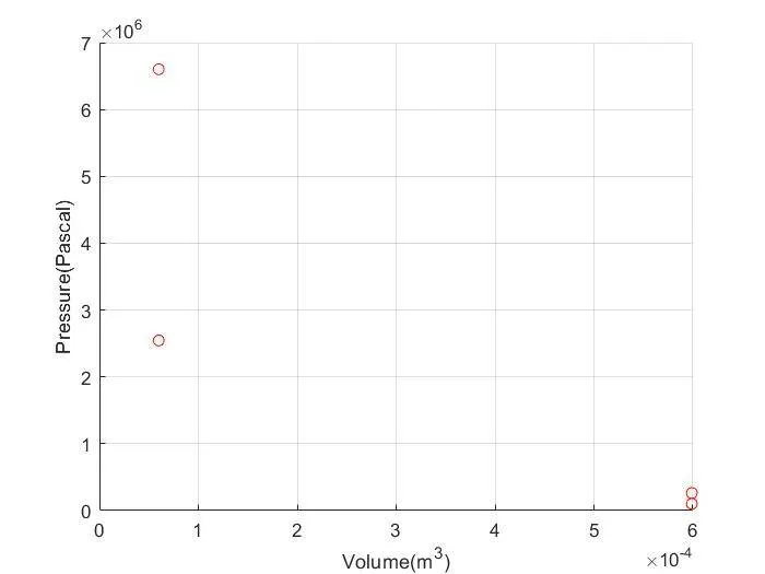
Figure4
Looks like the state points carry accurate reflections of our calculations.
Next, we will plot the process lines and display thermal efficiency.
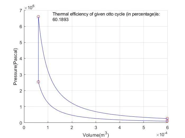
Figure5
So we have been able to obtain the required output.
Section6: Conclusion
The exercise for plotting otto cycle using MATLAB helped us to explore various features in MATLAB. We were successful in creating a user-defined function and use it in our plot. We have also learnt a method to display text on our graph. This concludes the challenge for writing a MATLAB code that can solve an otto cycle and make plots for it in the PV diagram while calculating and displaying the thermal efficiency of the engine.
References
1) https://www.researchgate.net/figure/Engine-geometry-and-parameters_tbl1_285745415