KNN (Breast Cancer) Prediction
import pandas as pd
import numpy as np
import seaborn as sns
import matplotlib.pyplot as plt
get_ipython().run_line_magic('matplotlib','inline')
# Get the data
from sklearn.datasets import load_breast_cancer
cancer=load_breast_cancer()
# Data set presenting in dictionary form
cancer.keys()
dict_keys(['data', 'target', 'frame', 'target_names', 'DESCR', 'feature_names', 'filename'])
print(cancer['DESCR'])
.. _breast_cancer_dataset:

Breast cancer wisconsin (diagnostic) dataset
--------------------------------------------

**Data Set Characteristics:**

    :Number of Instances: 569

    :Number of Attributes: 30 numeric, predictive attributes and the class

    :Attribute Information:
        - radius (mean of distances from center to points on the perimeter)
        - texture (standard deviation of gray-scale values)
        - perimeter
        - area
        - smoothness (local variation in radius lengths)
        - compactness (perimeter^2 / area - 1.0)
        - concavity (severity of concave portions of the contour)
        - concave points (number of concave portions of the contour)
        - symmetry
        - fractal dimension ("coastline approximation" - 1)

        The mean, standard error, and "worst" or largest (mean of the three
        worst/largest values) of these features were computed for each image,
        resulting in 30 features.  For instance, field 0 is Mean Radius, field
        10 is Radius SE, field 20 is Worst Radius.

        - class:
                - WDBC-Malignant
                - WDBC-Benign

    :Summary Statistics:

    ===================================== ====== ======
                                           Min    Max
    ===================================== ====== ======
    radius (mean):                        6.981  28.11
    texture (mean):                       9.71   39.28
    perimeter (mean):                     43.79  188.5
    area (mean):                          143.5  2501.0
    smoothness (mean):                    0.053  0.163
    compactness (mean):                   0.019  0.345
    concavity (mean):                     0.0    0.427
    concave points (mean):                0.0    0.201
    symmetry (mean):                      0.106  0.304
    fractal dimension (mean):             0.05   0.097
    radius (standard error):              0.112  2.873
    texture (standard error):             0.36   4.885
    perimeter (standard error):           0.757  21.98
    area (standard error):                6.802  542.2
    smoothness (standard error):          0.002  0.031
    compactness (standard error):         0.002  0.135
    concavity (standard error):           0.0    0.396
    concave points (standard error):      0.0    0.053
    symmetry (standard error):            0.008  0.079
    fractal dimension (standard error):   0.001  0.03
    radius (worst):                       7.93   36.04
    texture (worst):                      12.02  49.54
    perimeter (worst):                    50.41  251.2
    area (worst):                         185.2  4254.0
    smoothness (worst):                   0.071  0.223
    compactness (worst):                  0.027  1.058
    concavity (worst):                    0.0    1.252
    concave points (worst):               0.0    0.291
    symmetry (worst):                     0.156  0.664
    fractal dimension (worst):            0.055  0.208
    ===================================== ====== ======

    :Missing Attribute Values: None

    :Class Distribution: 212 - Malignant, 357 - Benign

    :Creator:  Dr. William H. Wolberg, W. Nick Street, Olvi L. Mangasarian

    :Donor: Nick Street

    :Date: November, 1995

This is a copy of UCI ML Breast Cancer Wisconsin (Diagnostic) datasets.
https://goo.gl/U2Uwz2

Features are computed from a digitized image of a fine needle
aspirate (FNA) of a breast mass.  They describe
characteristics of the cell nuclei present in the image.

Separating plane described above was obtained using
Multisurface Method-Tree (MSM-T) [K. P. Bennett, "Decision Tree
Construction Via Linear Programming." Proceedings of the 4th
Midwest Artificial Intelligence and Cognitive Science Society,
pp. 97-101, 1992], a classification method which uses linear
programming to construct a decision tree.  Relevant features
were selected using an exhaustive search in the space of 1-4
features and 1-3 separating planes.

The actual linear program used to obtain the separating plane
in the 3-dimensional space is that described in:
[K. P. Bennett and O. L. Mangasarian: "Robust Linear
Programming Discrimination of Two Linearly Inseparable Sets",
Optimization Methods and Software 1, 1992, 23-34].

This database is also available through the UW CS ftp server:

ftp ftp.cs.wisc.edu
cd math-prog/cpo-dataset/machine-learn/WDBC/

.. topic:: References

   - W.N. Street, W.H. Wolberg and O.L. Mangasarian. Nuclear feature extraction
     for breast tumor diagnosis. IS&T/SPIE 1993 International Symposium on
     Electronic Imaging: Science and Technology, volume 1905, pages 861-870,
     San Jose, CA, 1993.
   - O.L. Mangasarian, W.N. Street and W.H. Wolberg. Breast cancer diagnosis and
     prognosis via linear programming. Operations Research, 43(4), pages 570-577,
     July-August 1995.
   - W.H. Wolberg, W.N. Street, and O.L. Mangasarian. Machine learning techniques
     to diagnose breast cancer from fine-needle aspirates. Cancer Letters 77 (1994)
     163-171.
cancer['feature_names']
array(['mean radius', 'mean texture', 'mean perimeter', 'mean area',
       'mean smoothness', 'mean compactness', 'mean concavity',
       'mean concave points', 'mean symmetry', 'mean fractal dimension',
       'radius error', 'texture error', 'perimeter error', 'area error',
       'smoothness error', 'compactness error', 'concavity error',
       'concave points error', 'symmetry error',
       'fractal dimension error', 'worst radius', 'worst texture',
       'worst perimeter', 'worst area', 'worst smoothness',
       'worst compactness', 'worst concavity', 'worst concave points',
       'worst symmetry', 'worst fractal dimension'], dtype='<U23')
# Setup DataFrames
df_feat=pd.DataFrame(cancer['data'],columns=cancer['feature_names'])
df_feat.info()
<class 'pandas.core.frame.DataFrame'>
RangeIndex: 569 entries, 0 to 568
Data columns (total 30 columns):
 #   Column                   Non-Null Count  Dtype
---  ------                   --------------  -----
 0   mean radius              569 non-null    float64
 1   mean texture             569 non-null    float64
 2   mean perimeter           569 non-null    float64
 3   mean area                569 non-null    float64
 4   mean smoothness          569 non-null    float64
 5   mean compactness         569 non-null    float64
 6   mean concavity           569 non-null    float64
 7   mean concave points      569 non-null    float64
 8   mean symmetry            569 non-null    float64
 9   mean fractal dimension   569 non-null    float64
 10  radius error             569 non-null    float64
 11  texture error            569 non-null    float64
 12  perimeter error          569 non-null    float64
 13  area error               569 non-null    float64
 14  smoothness error         569 non-null    float64
 15  compactness error        569 non-null    float64
 16  concavity error          569 non-null    float64
 17  concave points error     569 non-null    float64
 18  symmetry error           569 non-null    float64
 19  fractal dimension error  569 non-null    float64
 20  worst radius             569 non-null    float64
 21  worst texture            569 non-null    float64
 22  worst perimeter          569 non-null    float64
 23  worst area               569 non-null    float64
 24  worst smoothness         569 non-null    float64
 25  worst compactness        569 non-null    float64
 26  worst concavity          569 non-null    float64
 27  worst concave points     569 non-null    float64
 28  worst symmetry           569 non-null    float64
 29  worst fractal dimension  569 non-null    float64
dtypes: float64(30)
memory usage: 133.5 KB
cancer['target']
array([0, 0, 0, 0, 0, 0, 0, 0, 0, 0, 0, 0, 0, 0, 0, 0, 0, 0, 0, 1, 1, 1,
       0, 0, 0, 0, 0, 0, 0, 0, 0, 0, 0, 0, 0, 0, 0, 1, 0, 0, 0, 0, 0, 0,
       0, 0, 1, 0, 1, 1, 1, 1, 1, 0, 0, 1, 0, 0, 1, 1, 1, 1, 0, 1, 0, 0,
       1, 1, 1, 1, 0, 1, 0, 0, 1, 0, 1, 0, 0, 1, 1, 1, 0, 0, 1, 0, 0, 0,
       1, 1, 1, 0, 1, 1, 0, 0, 1, 1, 1, 0, 0, 1, 1, 1, 1, 0, 1, 1, 0, 1,
       1, 1, 1, 1, 1, 1, 1, 0, 0, 0, 1, 0, 0, 1, 1, 1, 0, 0, 1, 0, 1, 0,
       0, 1, 0, 0, 1, 1, 0, 1, 1, 0, 1, 1, 1, 1, 0, 1, 1, 1, 1, 1, 1, 1,
       1, 1, 0, 1, 1, 1, 1, 0, 0, 1, 0, 1, 1, 0, 0, 1, 1, 0, 0, 1, 1, 1,
       1, 0, 1, 1, 0, 0, 0, 1, 0, 1, 0, 1, 1, 1, 0, 1, 1, 0, 0, 1, 0, 0,
       0, 0, 1, 0, 0, 0, 1, 0, 1, 0, 1, 1, 0, 1, 0, 0, 0, 0, 1, 1, 0, 0,
       1, 1, 1, 0, 1, 1, 1, 1, 1, 0, 0, 1, 1, 0, 1, 1, 0, 0, 1, 0, 1, 1,
       1, 1, 0, 1, 1, 1, 1, 1, 0, 1, 0, 0, 0, 0, 0, 0, 0, 0, 0, 0, 0, 0,
       0, 0, 1, 1, 1, 1, 1, 1, 0, 1, 0, 1, 1, 0, 1, 1, 0, 1, 0, 0, 1, 1,
       1, 1, 1, 1, 1, 1, 1, 1, 1, 1, 1, 0, 1, 1, 0, 1, 0, 1, 1, 1, 1, 1,
       1, 1, 1, 1, 1, 1, 1, 1, 1, 0, 1, 1, 1, 0, 1, 0, 1, 1, 1, 1, 0, 0,
       0, 1, 1, 1, 1, 0, 1, 0, 1, 0, 1, 1, 1, 0, 1, 1, 1, 1, 1, 1, 1, 0,
       0, 0, 1, 1, 1, 1, 1, 1, 1, 1, 1, 1, 1, 0, 0, 1, 0, 0, 0, 1, 0, 0,
       1, 1, 1, 1, 1, 0, 1, 1, 1, 1, 1, 0, 1, 1, 1, 0, 1, 1, 0, 0, 1, 1,
       1, 1, 1, 1, 0, 1, 1, 1, 1, 1, 1, 1, 0, 1, 1, 1, 1, 1, 0, 1, 1, 0,
       1, 1, 1, 1, 1, 1, 1, 1, 1, 1, 1, 1, 0, 1, 0, 0, 1, 0, 1, 1, 1, 1,
       1, 0, 1, 1, 0, 1, 0, 1, 1, 0, 1, 0, 1, 1, 1, 1, 1, 1, 1, 1, 0, 0,
       1, 1, 1, 1, 1, 1, 0, 1, 1, 1, 1, 1, 1, 1, 1, 1, 1, 0, 1, 1, 1, 1,
       1, 1, 1, 0, 1, 0, 1, 1, 0, 1, 1, 1, 1, 1, 0, 0, 1, 0, 1, 0, 1, 1,
       1, 1, 1, 0, 1, 1, 0, 1, 0, 1, 0, 0, 1, 1, 1, 0, 1, 1, 1, 1, 1, 1,
       1, 1, 1, 1, 1, 0, 1, 0, 0, 1, 1, 1, 1, 1, 1, 1, 1, 1, 1, 1, 1, 1,
       1, 1, 1, 1, 1, 1, 1, 1, 1, 1, 1, 1, 0, 0, 0, 0, 0, 0, 1])
df_target=pd.DataFrame(cancer['target'],columns=['Cancer'])
df_target.info()
df_feat.head()
| mean radius | mean texture | mean perimeter | mean area | mean smoothness | mean compactness | mean concavity | mean concave points | mean symmetry | mean fractal dimension | ... | worst radius | worst texture | worst perimeter | worst area | worst smoothness | worst compactness | worst concavity | worst concave points | worst symmetry | worst fractal dimension | |
|---|---|---|---|---|---|---|---|---|---|---|---|---|---|---|---|---|---|---|---|---|---|
| 0 | 17.99 | 10.38 | 122.80 | 1001.0 | 0.11840 | 0.27760 | 0.3001 | 0.14710 | 0.2419 | 0.07871 | ... | 25.38 | 17.33 | 184.60 | 2019.0 | 0.1622 | 0.6656 | 0.7119 | 0.2654 | 0.4601 | 0.11890 |
| 1 | 20.57 | 17.77 | 132.90 | 1326.0 | 0.08474 | 0.07864 | 0.0869 | 0.07017 | 0.1812 | 0.05667 | ... | 24.99 | 23.41 | 158.80 | 1956.0 | 0.1238 | 0.1866 | 0.2416 | 0.1860 | 0.2750 | 0.08902 |
| 2 | 19.69 | 21.25 | 130.00 | 1203.0 | 0.10960 | 0.15990 | 0.1974 | 0.12790 | 0.2069 | 0.05999 | ... | 23.57 | 25.53 | 152.50 | 1709.0 | 0.1444 | 0.4245 | 0.4504 | 0.2430 | 0.3613 | 0.08758 |
| 3 | 11.42 | 20.38 | 77.58 | 386.1 | 0.14250 | 0.28390 | 0.2414 | 0.10520 | 0.2597 | 0.09744 | ... | 14.91 | 26.50 | 98.87 | 567.7 | 0.2098 | 0.8663 | 0.6869 | 0.2575 | 0.6638 | 0.17300 |
| 4 | 20.29 | 14.34 | 135.10 | 1297.0 | 0.10030 | 0.13280 | 0.1980 | 0.10430 | 0.1809 | 0.05883 | ... | 22.54 | 16.67 | 152.20 | 1575.0 | 0.1374 | 0.2050 | 0.4000 | 0.1625 | 0.2364 | 0.07678 |
5 rows × 30 columns
#standardizing the variables
from sklearn.preprocessing import StandardScaler
scaler = StandardScaler()
scaler.fit(df_feat)
scaled_features=scaler.transform(df_feat)
df_feat_scaled=pd.DataFrame(scaled_features,columns=df_feat.columns)
df_feat_scaled.head()
| mean radius | mean texture | mean perimeter | mean area | mean smoothness | mean compactness | mean concavity | mean concave points | mean symmetry | mean fractal dimension | ... | worst radius | worst texture | worst perimeter | worst area | worst smoothness | worst compactness | worst concavity | worst concave points | worst symmetry | worst fractal dimension | |
|---|---|---|---|---|---|---|---|---|---|---|---|---|---|---|---|---|---|---|---|---|---|
| 0 | 1.097064 | -2.073335 | 1.269934 | 0.984375 | 1.568466 | 3.283515 | 2.652874 | 2.532475 | 2.217515 | 2.255747 | ... | 1.886690 | -1.359293 | 2.303601 | 2.001237 | 1.307686 | 2.616665 | 2.109526 | 2.296076 | 2.750622 | 1.937015 |
| 1 | 1.829821 | -0.353632 | 1.685955 | 1.908708 | -0.826962 | -0.487072 | -0.023846 | 0.548144 | 0.001392 | -0.868652 | ... | 1.805927 | -0.369203 | 1.535126 | 1.890489 | -0.375612 | -0.430444 | -0.146749 | 1.087084 | -0.243890 | 0.281190 |
| 2 | 1.579888 | 0.456187 | 1.566503 | 1.558884 | 0.942210 | 1.052926 | 1.363478 | 2.037231 | 0.939685 | -0.398008 | ... | 1.511870 | -0.023974 | 1.347475 | 1.456285 | 0.527407 | 1.082932 | 0.854974 | 1.955000 | 1.152255 | 0.201391 |
| 3 | -0.768909 | 0.253732 | -0.592687 | -0.764464 | 3.283553 | 3.402909 | 1.915897 | 1.451707 | 2.867383 | 4.910919 | ... | -0.281464 | 0.133984 | -0.249939 | -0.550021 | 3.394275 | 3.893397 | 1.989588 | 2.175786 | 6.046041 | 4.935010 |
| 4 | 1.750297 | -1.151816 | 1.776573 | 1.826229 | 0.280372 | 0.539340 | 1.371011 | 1.428493 | -0.009560 | -0.562450 | ... | 1.298575 | -1.466770 | 1.338539 | 1.220724 | 0.220556 | -0.313395 | 0.613179 | 0.729259 | -0.868353 | -0.397100 |
## Splitting the data into training and test data:
from sklearn.model_selection import train_test_split
X_train,X_test,y_train,y_test = train_test_split(scaled_features,np.ravel(df_target),test_size = 0.3,random_state = 105)
from sklearn.neighbors import KNeighborsClassifier
knn=KNeighborsClassifier(n_neighbors=1)
knn.fit(X_train,y_train)
pred=knn.predict(X_test)
# Predictions and Evaluations
from sklearn.metrics import classification_report,confusion_matrix
print(confusion_matrix(y_test,pred))
[[ 55   4]
 [  5 107]]
print(classification_report(y_test,pred))
              precision    recall  f1-score   support

           0       0.92      0.93      0.92        59
           1       0.96      0.96      0.96       112

    accuracy                           0.95       171
   macro avg       0.94      0.94      0.94       171
weighted avg       0.95      0.95      0.95       171
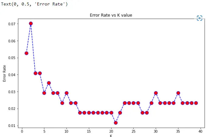
# Choosing a K value
error_rate=[]
for i in range(1,40):
knn=KNeighborsClassifier(n_neighbors=i)
knn.fit(X_train,y_train)
pred_i=knn.predict(X_test)
error_rate.append(np.mean(pred_i !=y_test))
plt.figure(figsize=(10,6))
plt.plot(range(1,40),error_rate,color='blue',linestyle='dashed',marker='o',
markerfacecolor='red',markersize=10)
plt.title('Error Rate vs K value')
plt.xlabel('K')
plt.ylabel('Error Rate')
# with K=1
knn=KNeighborsClassifier(n_neighbors=1)
knn.fit(X_train,y_train)
pred=knn.predict(X_test)
print('With K=1')
print('n')
print(confusion_matrix(y_test,pred))
print('n')
print(classification_report(y_test,pred))
With K=1


[[ 55   4]
 [  5 107]]


              precision    recall  f1-score   support

           0       0.92      0.93      0.92        59
           1       0.96      0.96      0.96       112

    accuracy                           0.95       171
   macro avg       0.94      0.94      0.94       171
weighted avg       0.95      0.95      0.95       171
# with K=21
knn=KNeighborsClassifier(n_neighbors= 21)
knn.fit(X_train,y_train)
pred=knn.predict(X_test)
print('With K=21')
print('n')
print(confusion_matrix(y_test,pred))
print('n')
print(classification_report(y_test,pred))
With K=21


[[ 57   2]
 [  0 112]]


              precision    recall  f1-score   support

           0       1.00      0.97      0.98        59
           1       0.98      1.00      0.99       112

    accuracy                           0.99       171
   macro avg       0.99      0.98      0.99       171
weighted avg       0.99      0.99      0.99       171