Genetic Algorithm

AIM

To apply the genetic algorithm for finding global maxima point in stalagmite function

OBJECTIVE

1) To write a code in MATLAB to optimize stalagmite function by applying a genetic algorithm for finding global maxima

2) explain the MATLAB code step by step and syntax of ga in MATLAB

3)performing studies with 3 types of conditions first unbounded condition, next bounded condition, and further bounded condition with increased population size

INTRODUCTION

Genetic Algorithm- The genetic algorithm is an evolutionary search-based algorithm based on Darwinism where its states fittest will survive the most. further, successive generations will become increasingly better than previous generations when compared to numerical methods each generation in the genetic algorithm is equal to each number of iterations. As the iteration count increases the optimization of the objective function(the function that needs to be maximized or minimized in an optimization problem) is improved similar way as generation count increases objective function improves in genetic algorithm.

Optimization- Finding out for which input values the function is optimized (according to needs minimization or maximization) and in some situations, it may take some constraints in to consideration for finding out the best(feasible) solution for those inputs.

For example- when it comes to electrical engineering, it is recommended to run a PV panel at maximum power point for economical reasons but for a partial shading condition the PV curve will be as shown in the figure below. Where there are small peaks (local maxima) points and one high peak (global maxima) point. When we use normal mathematical methods we would trap in those local points depending on the start region. So, this problem would require a global evolutionary optimization technique and the genetic algorithm is best suited for MPPT(maximum power point tracking).

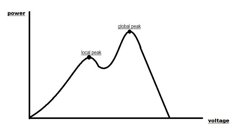
In a genetic algorithm, population means the number of feasible solutions(which are encoded), the chromosome is one of the solutions. Such that collection of all chromosomes will form the population and these solutions are encoded in some format and position of the encoding is one gene and fitness function is equal to the objective function.

There are some important operators for performing genetic algorithm and in stepwise Representation, Selection, Crossover and Mutation.

Representation- The way the data is represented and there are many ways like Binary, Real valued, Integer, Permutation based Representation

Selection - An individual from the current generation is selected based on fitness value and some technique is used to send them to the next generation as a parent. such that the fittest will only go to next-generation and some techniques used are Roulette wheel selection, Rank-based selection, Random selection, Stochastic universal sampling etc.

crossover - current generation selected parents are crossover to form an offspring(child) such that child gets both parents genes and there are many ways like one-point crossover, multipoint crossover, uniform crossover

Mutation - A single individual from the current generation undergoes some changes it can be done by techniques like Bit flip, Swap, Random resettling, Inversion etc.

Firstly, the population(number of solutions) are found then according to some technique the fitness value of each solution is estimated then according to the fitness value and selection technique some population(solutions) are selected and crossover is performed to those population to form off-spring(new set of solutions) and mutation is performed and this process is done until a feasible solution is obtained.

But, GA(genetic algorithm) is good for finding out the global optimal point but it is very slow in finding out the point. So, the best way is to use GA while starting an optimization problem when the GA enter the region of the Global maxima point then it is suggested to use some fast performing algorithms for finding our global optimal point and this is called the Hybrid optimization technique.

The syntax for GA in Matlab -

[x,fval,exitflag,output,population,scores] = ga(fun,nvars,A,b,Aeq,beq,lb,ub,nonlcon,intcon,options)

where, the code returns (x = minimum value), (fval = fitness function value at x(min value)),(exitflag = integer identifying the reason why algorithm terminated), (output = contains the output of each generation and about performace of algorithm), (final population) and (scores of final population)

and it takes inputs (fun = function which need to be optimized), (nvars = Number of variables), (A,B = Linear inequality constraints),(Aeq,beq=Linear equality constraints),(lb,ub= Lower and upper bounds),(nonlcon=Nonlinear constraints),(intcon=Integer variables) and (options=Optimization options which obtained by output of optimoptions)

Function need to be optimized (fitness function=(stalagmite function))

stagalmite function - `f1(x,y) = f1,x.f2,x.f1,y.f2,y`

where,

`f1,x = [sin(5.1pix+0.5)]^6` , `f2,x = exp[-4ln(2)(x-0.0667)^2/0.64]`

`f1,y = [sin(5.1piy+0.5)]^6` , `f2,y = exp[-4ln(2)(y-0.0667)^2/0.64]`

Matlab code for stalagmite function

function [f] = stalagmite(in_val)
        f1_x = (sin(5.1*pi*in_val(1)+0.5)).^6;
        f1_y = (sin(5.1*pi*in_val(2)+0.5)).^6;
        f2_x= exp(-4*log(2)*((in_val(1)-0.06667).^2)/0.64);
        f2_y = exp(-4*log(2)*((in_val(2)-0.06667).^2)/0.64);
        f = -(f1_x.*f2_x.*f1_y.*f2_y);
end

Optimization of function using ga

case-1 - unbounded condtion

without defining upper and lower bounds for inputs x and y

clear all
close all
clc
%defining search space
x = linspace(0,0.6,150);
y = linspace(0,0.6,150);
%number of times ga to run
num_cases = 50;
%creating 2-D array
[X,Y] = meshgrid(x,y);
%evaluating the stalagmite function
for i = 1:length(X)
    for j= 1:length(Y)
        input_vector(1)=X(i,j);
        input_vector(2) = Y(i,j);
        f(i,j) = stalagmite(input_vector);
    end
end
    
%study1 - unbounded condition
tic
for i = 1:num_cases
    %passing ga function where it takes inputs function, number of variables
    [inputs,fopt(i)] = ga(@stalagmite,2);
    xopt(i)=inputs(1);
    yopt(i)=inputs(2);
end
time_taken_study1 = toc;
figure(1)
subplot(2,1,1)
hold on
surfc(X,Y,-f)
shading interp
plot3(xopt,yopt,-fopt,'marker','o','markersize',3,'markerfacecolor','b')
title('unbounded condition')
xlabel('x value')
ylabel('y value')
grid on
subplot(2,1,2)
plot(-fopt)
xlabel('iterations')
ylabel('fmax')
toc
time_taken = toc

procedure and code explanation

• firstly a function is defined named stalagmite and we can call that into main code
• now, x and y inputs are given by use of linspace command
• then the iteration count i.e, how many times the ga algorithm is to be run is defined
• A 2-D array is created using meshgrid command
• then for inputs the stalagmite function is evaluated and using surfc command it is generated as surface plot
• now, using ga command the inputs to it (fitness function(stalagmite function)) and number of varibles supplied
• further, ga command gives out mimial optimal function value and inputs at optimal function value for getting maxima the function is multiplied by negitive sign
• then by using plot command a plot between fmax(maxmium value of function) and iterations is plotted in same figure

output

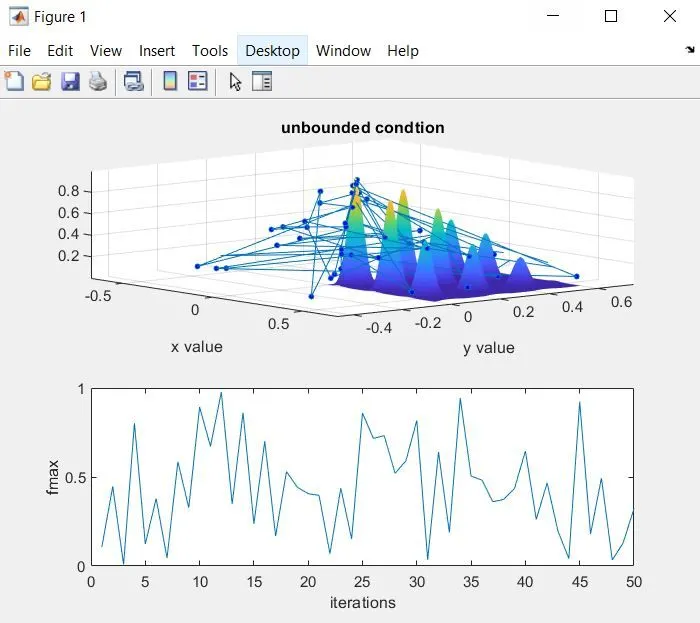
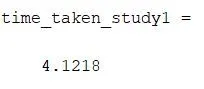
we can see the inputs are boundless such that genectic algorithm runs in unbounded search space

case-2 - bounded condtion

now defining the bounds for inputs lower bounds for x and y are 0,0 and upper bounds are 1,1

now the modified code is

clear all
close all
clc
%defining search space
x = linspace(0,0.6,150);
y = linspace(0,0.6,150);
%number of times ga to run
num_cases = 50;
%creating 2-D array
[X,Y] = meshgrid(x,y);
%evaluating the stalagmite function
for i = 1:length(X)
    for j= 1:length(Y)
        input_vector(1)=X(i,j);
        input_vector(2) = Y(i,j);
        f(i,j) = stalagmite(input_vector);
    end
end
%study 2-bounded_condition
tic
for j = 1:num_cases
    %now bounds are defined lower bounds 0,0 and upper bounds 1,1
    [inputs,fopt(j)] = ga(@stalagmite,2,[],[],[],[],[0;0],[1;1]);
    xopt(j)=inputs(1);
    yopt(j)=inputs(2);
end
time_taken_study2 = toc;

figure(2)
subplot(2,1,1)
hold on
surfc(X,Y,-f)
shading interp
plot3(xopt,yopt,-fopt,'marker','o','markersize',5,'markerfacecolor','r')
title('bounded condition')
xlabel('x value')
ylabel('y value')
grid on
subplot(2,1,2)
plot(-fopt)
xlabel('iterations')
ylabel('fmax')

output

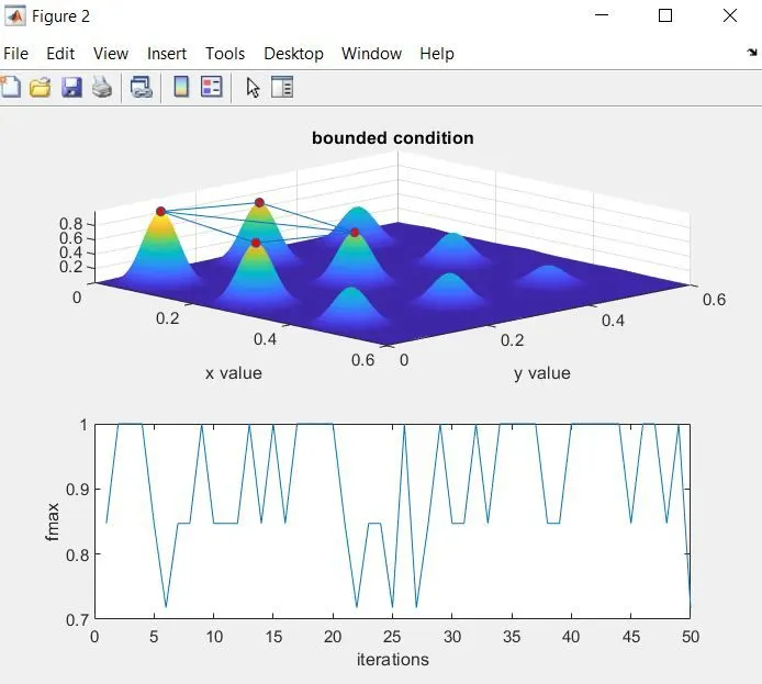
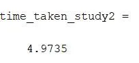
here as bounds are defined the ga algorithm search within boundaries but due to low population, it can be trapped at local minima points. So, by increasing population, it can converge to global maxima point.

case-3 - bounded condition with population defined

now population size is defined using optimoptions commad

clear all
close all
clc
%defining search space
x = linspace(0,0.6,150);
y = linspace(0,0.6,150);
%number of times ga to run
num_cases = 50;
%creating 2-D array
[X,Y] = meshgrid(x,y);
%evaluating the stalagmite function
for i = 1:length(X)
    for j= 1:length(Y)
        input_vector(1)=X(i,j);
        input_vector(2) = Y(i,j);
        f(i,j) = stalagmite(input_vector);
    end
end
%study 3-bounded with population size specified
options = optimoptions('ga','populationsize',300)
tic
for k = 1:num_cases
    [inputs,fopt(k)] = ga(@stalagmite,2,[],[],[],[],[0;0],[1;1],[],[],options);
    xopt(k)=inputs(1);
    yopt(k)=inputs(2);
end
time_taken_study3 = toc;
figure(3)
subplot(2,1,1)
hold on
surfc(X,Y,-f)
shading interp
plot3(xopt,yopt,-fopt,'marker','o','markersize',5,'markerfacecolor','r')
title('bounded condition with population size specified');
xlabel('x value')
ylabel('y value')
grid on
subplot(2,1,2)
plot(-fopt)
xlabel('iterations')
ylabel('fmax')
    
%study4
%options = optimoptions('ga','PlotFcn',@gaplotbestf,'populationsize',300)
%tic
%for l = 1:num_cases
    %[inputs,fopt(l)] = ga(@stalagmite,2,[],[],[],[],[0;0],[1;1],[],options);
    %xopt(l)=inputs(1);
    %yopt(l)=inputs(2);
%end
%time_taken_study3 = toc
%figure(4)
%subplot(2,1,1)
%hold on
%surfc(X,Y,-f)
%shading interp
%plot3(xopt,yopt,-fopt,'marker','o','markersize',5,'markerfacecolor','r')
%xlabel('x value')
%ylabel('y value')
%grid on
%subplot(2,1,2)
%plot(-fopt)
%xlabel('iterations')
%ylabel('fmax')

output

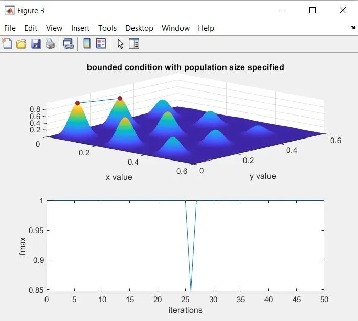
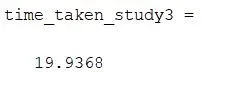
here, the variations are very less and ga able to track the global point for every single iteration in most cases

erros faced

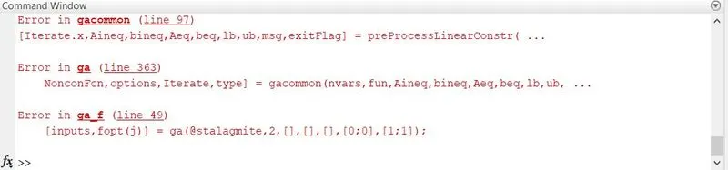
I made syntax error for ga further, the error is rectified

conslusion

So, it is observed that by increasing population count and defining boundries the genetic algrorithm will improve but the time taken to track will increase. So it is better to start with ga and then use any other faster search algorithm this technique is called hybrid optimization technique.

References-

1. P. Kumar, G. Jain and D. K. Palwalia, "Genetic algorithm based maximum power tracking in solar power generation," 2015 International Conference on Power and Advanced Control Engineering (ICPACE), 2015, pp. 1-6, doi: 10.1109/ICPACE.2015.7274907.
2. Mitchell, Melanie (1996). An Introduction to Genetic Algorithms. Cambridge, MA: MIT Press. ISBN 9780585030944
3. https://in.mathworks.com/help/gads/ga.html?s_tid=srchtitle_ga_1