Air standard Cycle- Otto cycle generation using MATLAB

AIM

To write a code in Matlab which solves the otto cycle and plot the PV diagram, also to output the thermal efficiency of the engine

THEORY

Otto cycle - It is an ideal thermodynamic cycle that represents the function of spark ignition reciprocating engine, it can be understood in 6 processes

1. (0-1) - intake stroke, at constant pressure air is taken into the piston
2. (1-2) - compression stroke, the air is compressed as the piston moves from the bottom dead centre(BDC) to the top dead centre(TDC). So, pressure and temperature increases and it is a reversible adiabatic process.
3. (2-3) - combustion, ignition is given to fuel-air mixture.
4. (3-4) - expansion stroke(power stroke), is a reversible adiabatic process.
5. (4-1) - heat rejection, heat is rejected at constant volume.
6. (1-0) - exhaust stroke, gases are released into the atmosphere at constant pressure.

Diagram

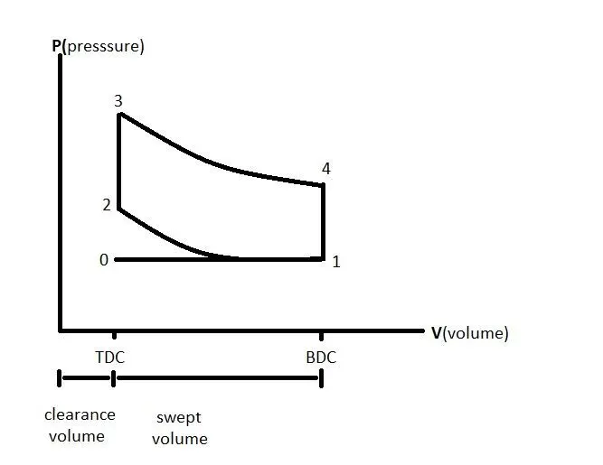
PV DIAGRAM FOR OTTO CYCLE

procedure

• we need the pressure and volume at 4 points to obtain the PV diagram for the otto cycle, we need the clearance and swept volume to obtain volume at point 1 and engine parameters like bore diameter, stroke length, compression ratio are needed to obtain swept and clearance volume, thus by temperature and volume at point1 pressure at point 1 can be calculated.
• by using the compression ratio volume at point 2 is calculated it is nothing but clearance volume. with help of the value of gamma, the pressure at point 2 is obtained by using the isentropic compression formula, thus the temperature by the ideal gas formula
• volume at point 3 doesn't change since (2-3) is a constant volume heat addition process, so (V2 = V3) and the pressure at point 3 calculated by taking the temperature at point 3 using the ideal gas formula.
• volume at point 4 is similar to the volume at point 1,(V4=V1) and pressure is calculated by isentropic compression formula

• now we obtained all 4 points in the PV diagram, to connect 4 points we need to know how volume varies between (1-2) and (3-4) this is known by piston kinematics which tells how piston moves from TDC TO BDC and how volume inside the piston changes this can be calculated by a geometrical formula

`V = Vc (1+0.5(cr-1)(R+1-costheta-(R^2-sin^2theta)^0.5)`

• where r is the ratio of connecting rod length to crankpin radius (a)
• The above formula is written as a function that can be recalled in the original otto cycle program for volume variation between (1-2) and (3-4), by this volume variations pressure variation between points (1-2) and (3-4) calculated by compression formula.
• thus the PV graph is generated by using the plot command

Efficiency

The thermal efficiency can be calculated by knowing the temperature at each state points by the formula

`eta = (1-((t4-t1)/(t3-t2)))*100`

MATLAB CODE

code for function

function [v] = engine_kinematics(bore,stroke,c_rod,cr,s_c_angle,e_c_angle)
 
%computing swept and clearance volume
v_swept = (pi/4)*((bore)^2)*stroke;
v_clearance = v_swept/(cr-1);
 
%how the volume in engine combustion chamber changes is given by formula
a = stroke/2; %crank pin radius
R = c_rod/a; 
theta = linspace(s_c_angle,e_c_angle,180); %in degree
 
term1 = 0.5*(cr-1);
term2 = R+1-cosd(theta);
term3 = (R^2 - sind(theta).^2).^0.5;
v = (1+term1*(term2-term3)).*v_clearance;
 
end

Main code

clear all
close all
clc
%inputs
gamma = 1.4;
a1 = 0;
a2 = 180;
%state variables
p1 = 101325; %assuming 1 atm written units in pascal
t1 = 500; %units in kelvin
t3= 2300; %units in kelvin
 
%engine geometric parameters
bore = 0.1;
stroke = 0.1;
c_rod = 0.15;
cr = 12;
 
%calculate the swept and clearance volume
v_swept = (pi/4)*((bore)^2)*stroke;
v_clearance = v_swept/(cr-1);
v1 = v_swept+v_clearance;
v2 = v_clearance;
 
%state variables at state point 2 
% p2*v2^gamma = p1*v1^gama isentropic compression formula
% p2 = p1*(v1/v2)^gamma, (v1/v2= compression ratio)
p2 = p1*cr^gamma;
%for temperature at state point 2 using ideal gas formula
% p1*v1/t2 = p2*v2/t2
t2 = p2*v2*t1/(p1*v1);
 
constant_c = p1*v1^gamma;
v_compression = engine_kinematics(bore,stroke,c_rod,cr,a2,a1); 
p_compression = constant_c./v_compression.^gamma;
 
%state variables at state point 3
%since state point 3 is end point of constant volume heat addition so
v3 = v2;
% for pressure use ideal gas law (p1*v1/t2 = p2*v2/t2)
p3 = p2*t3/t2;
 
constant_c = p3*v3^gamma;
v_expansion = engine_kinematics(bore,stroke,c_rod,cr,a1,a2); 
p_expansion = constant_c./v_expansion.^gamma;
 
%state variables at state point 4 
% volume at state point 4 is equal to volume at state 1 
v4 = v1;
% p3*v3^gama = p4*v4^gama (isentropic expansion/compression formula)
p4 = p3*(v3/v4)^gamma;
t4 = (p4*v4*t3)/(p3*v3);
figure(1)
hold on
plot(v1,p1,'*','color','r')
plot(v_compression,p_compression,'color','b');
plot(v2,p2,'*','color','r')
plot(v3,p3,'*','color','r')
plot(v_expansion,p_expansion,'color','b')
plot(v4,p4,'*','color','r')
plot([v2 v3],[p2 p3],'color','b')
plot([v1 v4],[p1 p4],'color','b')
xlabel('volume');
ylabel('pressure');
title('pressure vs volume curve');
fprintf(' volume and pressure at state point 1 are %d, %d n',v1',p1);
fprintf(' volume and pressure at state point 2 are %d, %d n',v2',p2);
fprintf('volume and pressure at state point 3 are %d, %d n',v3',p3);
fprintf('volume and pressure at state point 4 are %d, %d n',v4',p4);
effi = (1-((t4-t1)/(t3-t2)))*100;
fprintf('thermal efficiency in percentage is %f',effi);

OUTPUT

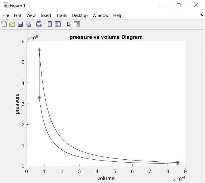
errors faced

first while using fprintf command I didn't use slash n at the end so all outputs printed in one line

CONCLUSION

The otto cycle PV diagram is generated using Matlab and thus the thermal efficiency is calculated