Curve fitting using matlab

AIM

To write a Matlab program to fit curve for the given Cp data by considering linear and cubic polynomial and measure the fitness characteristics of curves.

THEORY

curve fitting- it is a method used to extract the output for certain input which is not given in data by constructing a graphical curve for given data set. the curve is constructed by assuming a mathematical polynomial function of any order then finding out the coefficients of the function assumed using the data set by using interpolation. it is very useful for forecasting an output with the help of past data samples, it has applications in data analytics where one need to visualise the data graphically

there are many curve-fitting techniques we are using polynomial curve fit this can be further classified to

-linear fit is nothing but using 1st order polynomial equation nothing but the fitting straight line in the data this is used when we don't know the relation between the input and output of data given. `y= ax+b`

-cubic polynomial fit is used when the curve bends more than two times, the relation between the inputs and output is expected to be a polynomial with the power of 3. `y= ax^3+bx^2+cx+d`

measuring the fitness of the curve

the error between the curve obtained by data and the curve fitted is minimum such that the best fit is obtained. to obtain the perfect fit we need the error to be zero error can be measured in different ways they are

1. square errors due to error- it measures the total deviation of the response values from the fit to the response values, as value close to zero the better fit. it also called as sum of squared errors(SSE) `SSE = sum_(i=0)^n err(i)^2`
2. R-square - R-square is the square of the correlation between the response values and the predicted response values, it outputs values between 0 and 1 as the fit is close to 1 the better fit and low error. R square defined as the ratio of the sum of squares of regression(SSR) to the total sum of squares(SST) `R^2 = (SSR)/(SST)`
3. adjusted R-square- here the above R-square is adjusted according to the residual degree of freedom which means the number of response values n minus the number of fitted coefficients m estimated from the response values and given by `R^2adj = 1-[((1-R^2)(n-1))/(n-k-1)]` where n = number of data points, k= number of independent variables
4. root mean squared error- it is also called the standard error of regression and it is defined as the square root of ratio to sum of square errors(SSE) to total number of data points available `RSME = sqrt ((SSE)/n)`

procedure

- open Matlab editor then first we need to give commands clear all, close all,clc then the data need to be loaded it is done by command load then followed by file name in brackets and it is assigned to cp_data where the temperature is in 1st column and corresponding specific heat in 2nd column of the file

-then we use polyfit command which takes x and y coordinates and degree of the polynomial and gives the coefficient values of the equation the the predicted specific heat curve for different temperature is obtained by polyval command which takes coefficients and temperature as input

- then by using the plot command the plots for both specific heat and predicted specific heat is plotted for different temperature values

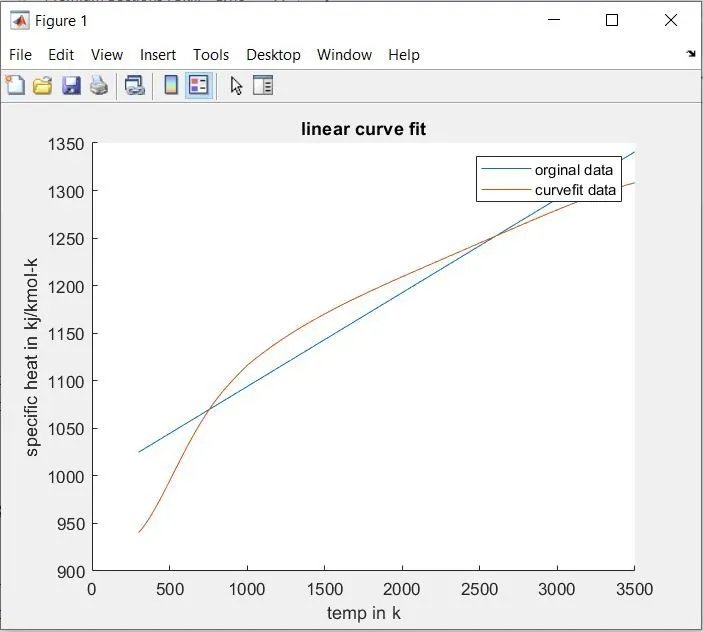
for linear fit - the degree of the polynomial is given as 1 and then the curve is plotted

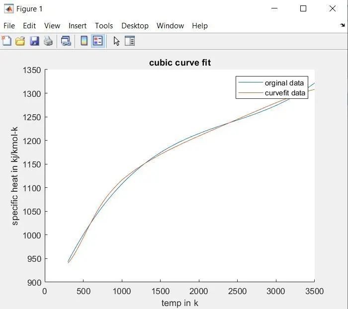
for cubic fit - the degree of the polynomial is taken as 3 and then the curve is plotted

code for the linear fit

%preparing the data
cp_data = load('data');
temp = cp_data(:,1);
cp = cp_data(:,2);

%curvefit
%cp = a*t+b;
co_eff = polyfit(temp,cp,1);
predicted_cp = polyval(co_eff,temp);

%compare
hold on
plot(temp,predicted_cp);
plot(temp,cp);
xlabel('temp in k');
ylabel('specific heat in kj/kmol-k');
legend('orginal data','curvefit data');
title('linear curve fit');

plotted curve for the linear fit

code for cubic fit

clear all
close all
clc
%preparing the data
cp_data = load('data');
temp = cp_data(:,1);
cp = cp_data(:,2);

%curvefit
%cp = a*t^3+b*t^2+c*t+c;
co_eff = polyfit(temp,cp,3);
predicted_cp = polyval(co_eff,temp);

%compare
hold on
plot(temp,predicted_cp);
plot(temp,cp);
xlabel('temp in k');
ylabel('specific heat in kj/kmol-k');
legend('orginal data','curvefit data');
title('cubic curve fit');

by using the above code we get a warning message as 'Polynomial is badly conditioned. Add points with distinct X values, reduce the degree of the polynomial, or try centring and scaling as described in HELP POLYFIT'

to overcome this issue we need to do centring and scaling this can be done by the below code. it improves the numerical properties of the problem. polyfit centres the data in temperature at 0 and scales it to have a standard deviation of 1

clear all
close all
clc

%preparing the data
cp_data = load('data');
temp = cp_data(:,1);
cp = cp_data(:,2);

%curvefit
%cp = a*t+b;
[co_eff,S,mu] = polyfit(temp,cp,3);
predicted_cp = polyval(co_eff,temp,S,mu);

%compare
hold on
plot(temp,predicted_cp);
plot(temp,cp);
xlabel('temp in k');
ylabel('specific heat in kj/kmol-k');
legend('orginal data','curvefit data');
title('cubic curve fit');

plotted curve for cubic fit

evaluating fitness by curve fit toolbox

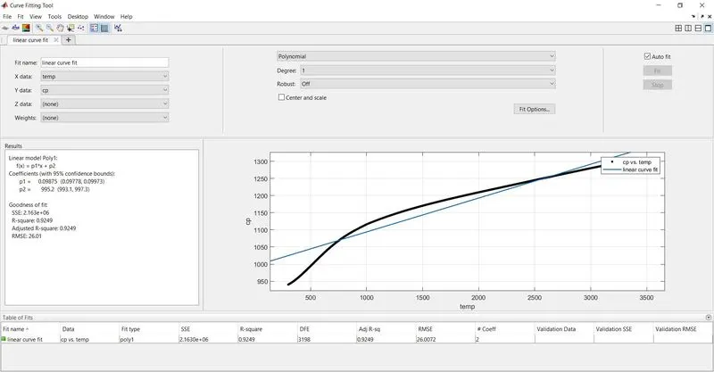
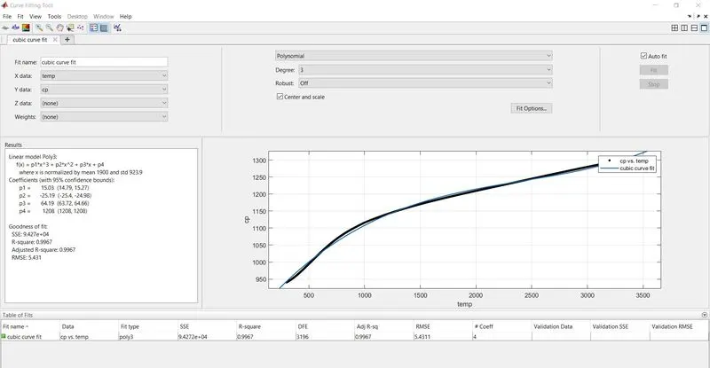
curve fit toolbox in Matlab can obtain the curve without writing any code and it also outputs the fitness of the curve

for linear fit

for cubic fit

split wise method

here when we know the variation of data for particular intervals then we split data into intervals and then for those intervals we use polynomial curve fit which help us to fit the curve better way here data is split into 4 intervals in 1st interval from 0 to 1000 k temperature and for 1001 to 1500, 1501 to 2500,2501 to 3200. as the variation between 1501 to 2500 is linear so we use linear curve fit here and other parts use 2nd order polynomial curve fit since it has some bendings

clear all
close all
clc

%preparing the data
cp_data = load('data');
temp = cp_data(:,1);
cp = cp_data(:,2);

temp1 = cp_data(1:1000,1);
cp1 = cp_data(1:1000,2);

temp2 = cp_data(1001:1500,1);
cp2 = cp_data(1001:1500,2);

temp3 = cp_data(1501:2500,1);
cp3 = cp_data(1501:2500,2)

temp4 = cp_data(2501:3200,1);
cp4 = cp_data(2501:3200,2);


%curvefit
%cp = a*t^2+b*t+c
co_eff1 = polyfit(temp1,cp1,2);
predicted_cp1 = polyval(co_eff1,temp1);
%cp = a*t^2+b*t+c
co_eff2 = polyfit(temp2,cp2,2);
predicted_cp2 = polyval(co_eff2,temp2);
%cp = a*t+b
co_eff3 = polyfit(temp3,cp3,1);
predicted_cp3 = polyval(co_eff3,temp3);
%cp = a*t^2+b*t+c
co_eff4 = polyfit(temp4,cp4,2);
predicted_cp4 = polyval(co_eff4,temp4);

%compare
hold on
plot(temp,cp,'color','r','linewidth',2);
plot(temp1,predicted_cp1,'color','b','linewidth',2);
plot(temp2,predicted_cp2,'color','b','linewidth',2);
plot(temp3,predicted_cp3,'color','b','linewidth',2);
plot(temp4,predicted_cp4,'color','b','linewidth',2);
xlabel('temp in k');
ylabel('specific heat in kj/kmol-k');
legend('orginal data','curvefit data');
title('split wise curve fit');

obtained curve fit with the above code

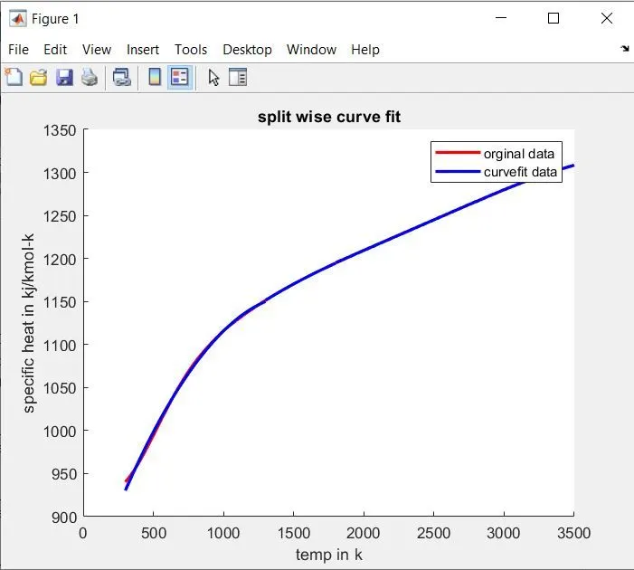
here we can see the curve is fitted more accurately

conclusion

the linear and cubic polynomial curve fit is performed for given data and measured the fitness of curve then used split wise method for the data which fitted curve with low error