Genetic Algorithm

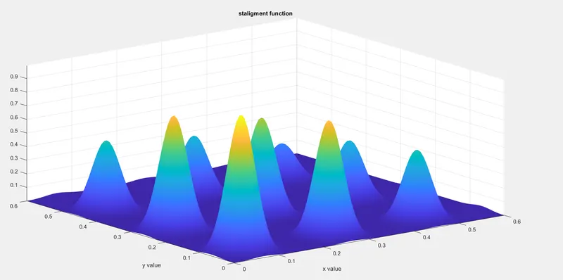
AIM: code in MATLAB to optimize the stalagmite function and find the global maxima of the function.

introduction: Genetic Algorithm is basically an optimization technique used to solve non-linear or non-differentiable
optimization problems, they use concepts from evolutionary biology to search for a global minimum to an optimization problem.
the name genetic algorithm comes from the fact that their mimicking evolutionary biology techniques.
to give a proper definition for GA, we can say that it is an optimization technique used get values so that we can get the best
output values or results. steps involved are:
1. initialization
2. fitness assignment
3. selection
4. cross over
5. mutation
6. stopping criteria

SYNTAX FOR GA:

x = ga(fun,nvars,A,b,Aeq,beq,lb,ub)

where

x is the optimum solution.

nvars is number of variables

A,b are linear inequality constraints

Aeq,beq are linear equality constraints

lb is upper bound

ub is upper bound

note: GA is only used to generate a minimum solution. so the value of stalagmite function
is taken negatively to maximize the function.

#Code for stalagmite function#

function [F] = stalagmite(input_vec)
x=input_vec(1)
y=input_vec(2)

f1_x = (sin(5.1*pi*x+0.5)).^6;
f1_y = (sin(5.1*pi*y+0.5)).^6;
f2_x = exp(-4*log(2)*(x-0.0667).^2)/0.64);
f2_y = exp(-4*log(2)*(y-0.0667).^2)/0.64);
[F] = -(f1_x.*f1_y.*f2_x.*f2_y);
end

#code to find the global maxima of the function#

clear all
close all
clc

%code to find the global maxima of the function#
 
%creating x and y array
 
x=linspace(0,0.6,150);
y=linspace(0,0.6,150);
num_cases=50;
[xx,yy]=meshgrid(x,y);
 
%calculating the stalagmite function
for i=1:length(xx)
   for j=1:length(yy)
       input_vector(1)=xx(i,j);
       input_vector(2)=yy(i,j);
       f(i,j)=stalagmite_func(input_vector);
    end
end
%createing 3D surface
figure(1)
surfc(xx,yy,-f)
shading interp
xlabel('x value')
ylabel('y value')
title('staligment function')
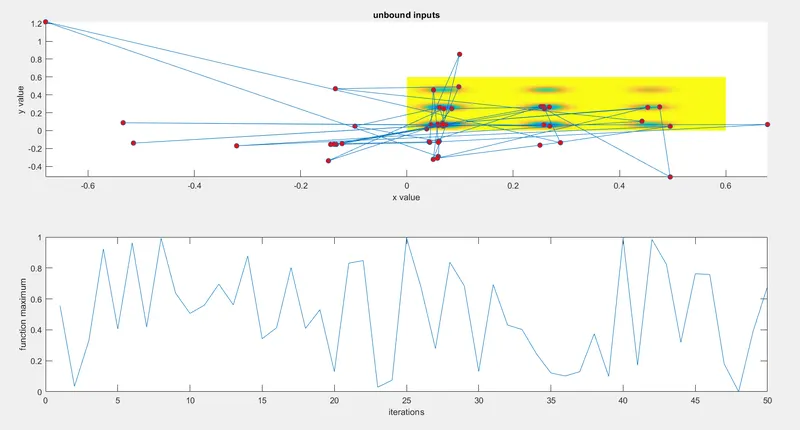
%study one
tic
for i = 1:num_cases
    [inputs,fopt(i)]=ga(@stalagmite_func,2);
    xopt(i)=inputs(1);
    yopt(i)=inputs(2);
end
study_1 = toc
figure(2)
subplot(2,1,1)
hold on
surfc(x,y,f)
title('unbound inputs')
xlabel('x value')
ylabel('y value')

shading interp
hold on

plot3(xopt,yopt,-fopt,'marker','o','markerfacecolor','r')
subplot(2,1,2)
plot(-fopt)
xlabel('iterations')
ylabel('function maximum')

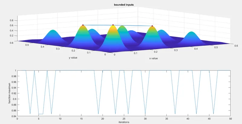
%study 2

tic;
for i=1:num_cases
    [inputs,fopt(i)]=ga(@stalagmite_func,2,[],[],[],[],[0;0],[0.6;0.6]);
    xopt(i)=inputs(1);
    yopt(i)=inputs(2);
end

study_2_time=toc
figure(3)
subplot(2,1,1)
surfc(x,y,-f)
shading interp
title('bounded inputs')
xlabel('x value')
ylabel('y value')

hold on
plot3(xopt,yopt,-fopt,'marker','o','markersize',5,'markerfacecolor','r')
subplot(2,1,2)
plot(-fopt)
xlabel('iterations')
ylabel('function maximun')

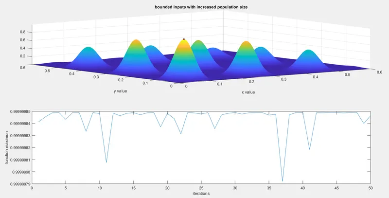
%Study 3 increasing the population size
%here we are increasing the probablity of the function
%converge at global maximum

options=optimoptions(@ga)
options=optimoptions(@ga,'populationsize',500)

tic
for i =1:num_cases
   [inputs,fopt(i)]=ga(@stalagmite_func,2,[],[],[],[],[0;0],[0.6;0.6],[],[],options);
   xopt(i)=inputs(1);
   yopt(i)=inputs(2);
end
study_3_time = toc
figure(4)
subplot(2,1,1)
surfc(x,y,-f)
shading interp
title('bounded inputs with increased population size')
xlabel('x value')
ylabel('y value')

hold on

plot3(xopt,yopt,-fopt,'marker','o','markersize',4,'markerfacecolor','r')
subplot(2,1,2)
plot(-fopt)
xlabel('iterations')
ylabel('function maximun')

result:

study_1_time =

2.1270

study_2_time =

2.6355

study_3_time =

16.4686