Curve fitting using Splitwise method

AIM: To write a program in Matlab for curve fitting using split-wise method

Parameters used to measure the fitness characteristics of the curve:

1. the sum of square due to error
2. R-square
3. Adjusted R-square
4. Root mean square error
in this project, we will only talk about R-square error and for R-square, if it is greater than 0.95 then the fit is assumed to be good.

Governing Equations:

R^2 = SSR/SST
where SSR is sum of squares of regression
and SST is summation for SSR AND SSE (SST = SSE + SSR)
SSE is sum of squares due to error

OBJECTIVE:
1. plot curve fit for a linear and cubic polynomial
2. verify the fitness of the curve using the split-wise method.

code for curve fitting using linear and cubic polynomial:

clear all
close all
clc

%preparing data 
cp_data = load('data');
%load command is used to read the file
temperature = cp_data (:,1);
%we are saving temperature here as the first column of the cp_data
cp = cp_data(:,2);
%plot
plot (temperature,cp,'linewidth',3)
xlabel('Temperature [K]')
ylabel('specific heat [KJ/Kmol-K]')

%curve fit for linear 
 
%cp_1 = a*T + b
co_effs1 = polyfit(temperature,cp,1);
predicted_cp = polyval(co_effs1,temperature);

%to compare my curve fit with the original data
plot(temperature,cp,'linewidth',3)
hold on
plot(temperature,predicted_cp,'linewidth',3,'color','r')
xlabel('Temperature [K]')
ylabel('Specific Heat [KJ/Kmol-K]')
legend('original dataset','curve fit')
title('specific heat vs temperature [for linear curve fitting]')

%parameter [R square] to validate best fit

total_cp = 0;
for i = 1: length(cp_data(:,1))
total_cp = total_cp +cp(i); %calculating all summation of cp
end

mean = total_cp/3200; 
%this gives mean of cp values
%for R Square we need to calculate SSR and SSE
SSR=0;
for j = 1: length(cp_data(:,1))
SSR=SSR+(predicted_cp(j) - mean)^2;
end

SSE=0;
for k =1:length(cp_data(:,2))
SSE = SSE +(cp(k) - predicted_cp(k))^2;
end

R_square_linear = (SSR/(SSR+SSE));
if R_square_linear >= 0.95
RESULT_1 = sprintf('linear curve fitting is good')
else RESULT_1 = sprintf('linear curve fitting is not good')
end


%curve fit for cubic
figure(2)
%cp_2 = a*T^3 + b*T^2 + c^T + d
co_effs2 = polyfit(temperature,cp,3);
predicted_cp3 = polyval(co_effs2,temperature);
%to compare my curve fit with the original data
plot(temperature,cp,'linewidth',3)
hold on
plot(temperature,predicted_cp3,'linewidth',3,'color','r')
xlabel('Temperature [K]')
ylabel('Specific Heat [KJ/Kmol-K]')
legend('original dataset','curve fit')
title('specific heat vs temperature [for cubic curve fitting]')

%to calculate SSE and SSR for cubic curve fit
SSR_3 = 0;
for m =1: length(cp_data(:,1))
SSR_3 = SSR_3 + (predicted_cp3(m) - mean)^2;
end

SSE_3 = 0;
for n=1: length(cp_data(:,1))
SSE_3 = SSE_3 + (cp(n) - predicted_cp3(n))^2;
end

R_square_cubic = (SSR_3 /(SSR_3 + SSE_3));

if R_square_cubic >= 0.95
Result_2 = sprintf('CUBIC CURVE FITTING IS GOOD')
else RESULT_2 = sprintf('CUBIC CURVE FITTING IS NOT GOOD')
end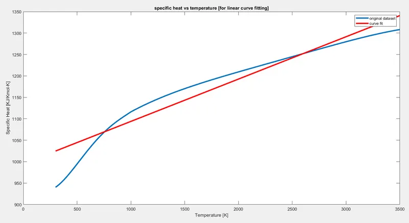

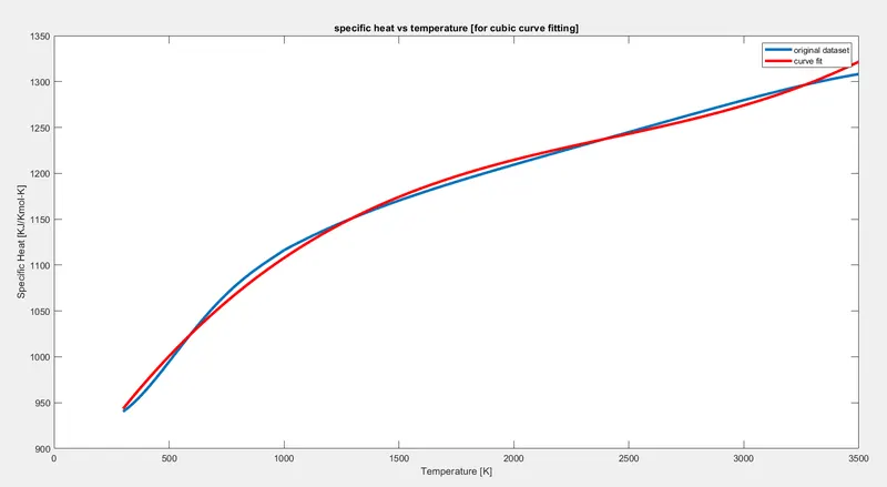
Result: (of the linear and cubic curve)
by observing these plots, we can conclude that the cube curve fitting is better than the linear curve fitting. and now to be sure we can R square method.
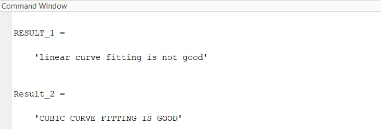
here using the R square method we got to know that the curve fitting is good as the value of it is more than 0.95

Based on the following conclusions, let us answer few questions now.

How to make a curve fit perfectly?
without showing the centering error and scaling error we need to fir the curve the original curve. we can improvise a perfect fit by minimizing error and making it to be the best fit.
a perfect fit can always be the best fit but the best fit can not be the perfect fit always.

How to get the best fit?
as we already have understood that perfect fir and best fit are two different phenomena, let us continue.
to get the best fit we can check the parameters of the curve fitting and also increase the order of the polynomial to get the best fit. and also in some cases, we can use split wise method to get the best fit.

What should we do to improve the cubic fit?
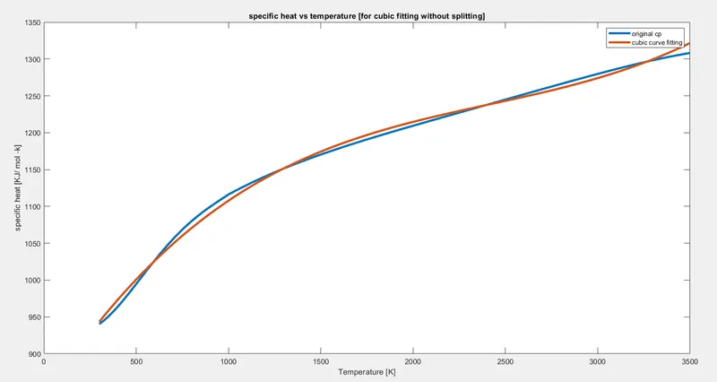
by using the split-wise method we can improve the curve fit. we should split the original data into smaller sections and compute the co-effs for the curve fits for different sections of data. and in the end, we can combine these values and plot over the entire data.

The first part is done, now let us move to the second part where we improvise the curve fitting of the cubic polynomial which is done by using the split-wise method.

clear all
close all
clc

%program for curve fitting

x= load('data'); 
temp =x(:,1);
cp =x(:,2);

%code for q curve fitting with split

%cp =  a*temp^3 +b*temp^2 + c*temp + d

temp_1 = temp(1:800); %temperature values fro split 1
temp_2 = temp(801:1600); %temperature values fro split 2
temp_3 = temp(1601:2400); %temperature values fro split 3
temp_4 = temp(2401:3200); %temperature values fro split 4

cp_1 = cp(1:800); %specific heat values fro split 1
cp_2 = cp(801:1600); %specific heat values fro split 2
cp_3 = cp(1601:2400); %specific heat values fro split 3
cp_4 = cp(2401:3200); %specific heat values fro split 4

co_eff = polyfit(temp,cp,3);
predicted_cp = polyval(co_eff,temp);

co_eff1= polyfit(temp_1,cp_1,2);
predicted_cp_1= polyval(co_eff1,temp_1);

co_eff2= polyfit(temp_2,cp_2,2);
predicted_cp_2= polyval(co_eff2,temp_2);

co_eff3= polyfit(temp_3,cp_3,2);
predicted_cp_3= polyval(co_eff3,temp_3);

co_eff4= polyfit(temp_4,cp_4,2);
predicted_cp_4= polyval(co_eff4,temp_4);

%plotting for fig(1)

figure(1);
plot(temp,cp,'linewidth',3);
hold on
plot(temp,predicted_cp,'linewidth',3);
xlabel('Temperature [K]');
ylabel('specific heat [KJ/ mol -k]');
legend('original cp','cubic curve fitting')
title('specific heat vs temperature [for cubic fitting without splitting]')
hold off

%plot for cubic curve without splitting
%plotting for figure (2)

figure(2);
plot(temp,cp,'linewidth',3);
hold on
plot(temp_1,predicted_cp_1,'linewidth',3);
plot(temp_2,predicted_cp_2,'linewidth',3);
plot(temp_3,predicted_cp_3,'linewidth',3);
plot(temp_4,predicted_cp_4,'linewidth',3);
xlabel('temperature [k]');
ylabel('specific heat [KJ/mol=k]')
legend('original cp','cubic curve fitting')
title('specific heat vs temperature [for cubic curve fitting with splitting]')
hold off

%parameter[R-Square] to validate best fitting:

Total_cp = 0; 
for i = 1:800
    Total_cp_1= Total_cp + cp_1(i); %to calculate summation of cp values for 1st split
    Total_cp_2= Total_cp + cp_2(i); %to calculate summation of cp values for 2nd split
    Total_cp_3= Total_cp + cp_3(i); %to calculate summation of cp values for 3rd split
    Total_cp_4= Total_cp + cp_4(i); %to calculate summation of cp values for 4th split
end

mean_1 = Total_cp_1 / 800; %to calculate mean cp 
mean_2 = Total_cp_2 / 800; %to calculate mean cp 
mean_3 = Total_cp_3 / 800; %to calculate mean cp 
mean_4 = Total_cp_4 / 800; %to calculate mean cp 

%to calculate sum of square of the regression [SSR]

SSR=0;
for m = 1:800
    SSR = SSR + (predicted_cp_1(m) - mean_1)^2;
    SSR = SSR + (predicted_cp_2(m) - mean_2)^2;
    SSR = SSR + (predicted_cp_3(m) - mean_3)^2;
    SSR = SSR + (predicted_cp_4(m) - mean_4)^2;
end
%to calculate sum of squared errors[SSE]

SSE=0;
for n = 1:800
    SSE = SSE+(cp_1(n) - predicted_cp_1(n))^2;
    SSE = SSE+(cp_2(n) - predicted_cp_2(n))^2;
    SSE = SSE+(cp_3(n) - predicted_cp_3(n))^2;
    SSE = SSE+(cp_4(n) - predicted_cp_4(n))^2;
end
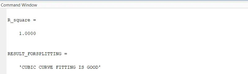
R_square = (SSR / (SSR+SSE))

if R_square >= 0.95
 RESULT_FORSPLITTING = sprintf ('CUBIC CURVE FITTING IS GOOD')
else RESULT_FOR_SPLITTING = sprintf('CUBIC CURVE FITTING IS NOT GOOD')
end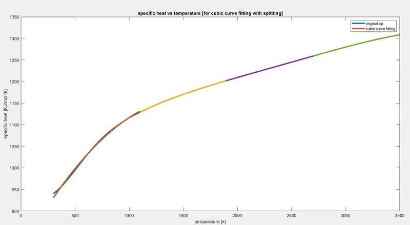

conclusion:
R square value for linear curve fit: 0.924877626055183
R square value for cubic curve fit: 0.996725946714054
so we concluded that the linear curve fit is not a good fit
then we further improved the curve fit of the cubic curve fit by using a split-wise method where the R square value was 1. so we have given the best fit for the curve fit.