Air standard Cycle PV Diagram and Thermal efficiency

Objective: To generate a program to create a PV diagram and to find the thermal efficiency of Otto cycle.

Governing equations:

1. v_swept=(pi/4)*bore^2*stroke

2. v_clearance=v_swept/(cr-1)

3. v1=v_swept+v_clearance

4. v2=v_clearance

5. p2v2^gamma=p1v1^gamma

6. t2=p2*v2*t1/(p1*v1)

7. p3v3/t3=p2v2/t2

8. p3v3^gamma=p4v4^gamma

9. termal_efficiency= 1-(cr)^(1-gamma)

where v_swept is the volume of the cylinder which can be determined with respect to bore and stroke; v_clearance is clearance volume which is the ratio of swept volume to (cr-1) where cr is clearance ratio = 12. p1,v1,t1 are pressure, volume, and temperate at state point one. similarly, p2,v2,t2 are pressure, volume, and temperate at state point two, etc.,

Body:

code: (i) for otto cycle PV diagram and Thermal efficiency

clear all
close all
clc

%inputs 

gamma = 1.4;
t3 = 2500;

%state variables

p1=101325; %atm pressure
t1=500;

%engine geometric parameters

bore = 0.1;
stroke = 0.1;
con_rod=0.15;
cr=12;

%calculating the swept and clearance volume

v_swept=(pi/4)*bore^2*stroke;
v_clearance=v_swept/(cr-1);
v1=v_swept+v_clearance;
v2=v_clearance;

%state variables at point 2

%p2v2^gamma=p1v1^gamma
p2=p1*cr^gamma;
%t2=p2*v2*t1/(p1*v1)
t2= p2*v2*t1/(p1*v1);
constant_c=p1*v1^gamma;
v_compression=engine_kinematics(bore,stroke,con_rod,cr,180,0);
p_compression=constant_c./v_compression.^gamma;

%state variables at state point 3

v3=v2;
%p3v3/t3=p2v2/t2 | p3=p2*t3/t2
p3=p2*t3/t2;
constant_c=p3*v3^gamma;
v_expantion= engine_kinematics(bore,stroke,con_rod,cr,0,180);
p_expantion=constant_c./v_expantion.^gamma;

%state variables at point 4

v4=v1;
%p3v3^gamma=p4v4^gamma | p4=p3*(v3/v4)^gamma
p4=p3*(v3/v4)^gamma;
t4=p4*v4*t3/(p3*v3);
termal_efficiency= 1-(cr)^(1-gamma)
figure(1);
hold on 
%plotting
plot (v1,p1,'*','color','r')
plot(v_compression,p_compression)
plot (v2,p2,'*','color','r')
plot([v2,v3],[p2,p3],'color','b') %straight vertical line (constant volume heat addition)
plot (v3,p3,'*','color','r')
plot(v_expantion,p_expantion)
plot (v4,p4,'*','color','r')
plot([v4,v1],[p4,p1],'color','b') %straight vertical line (constant volume heat rejection)
xlabel('Volume')
ylabel('Pressure')

(ii) to define and call a function "engine_kinematics"

function [v] = engine_kinematics(bore,stroke,con_rod,cr,start_crank,end_crank)

a = stroke/2;
R = con_rod/a;
v_s = pi/4*bore^2*stroke;
v_c = v_s/(cr-1);

theta = linspace(start_crank,end_crank,100);

term1 = 0.5*(cr-1);
term2 = R+1 - cosd(theta);
term3 = (R^2 - sind(theta).^2).^0.5;
v = (1+term1*(term2 - term3)).*v_c;
end

Result:

thermal efficiency = 0.6299 = 62.99 %

PV_diagram:

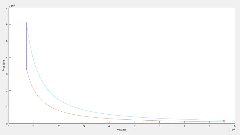
we can see the PV diagram plotted where the process 1 to 2 which is represented by the orange line is isentropic compression and process 2 to 3 which is a vertical dark blue line on the left represents constant volume heat addition. Process 3 to 4 on top (light blue line) represents the isentropic expansion and process 4 to 1 represents constant volume heat rejection.