Gearbox sloshing effect
Question
For this challenge, you have to perform the four simulations in the Gearbox and then you have to compare the results among all the four cases.
Part 1:
- 20% Immersion, Fluid - Engine oil.
- 30% Immersion, Fluid- Engine oil.
- 20% Immersion,Fluid-n-heptane (c7h16).
- 30% Immersion,Fluid-n-heptane (c7h16).
Part 2:
- What is Dynamic meshing? Give some other examples where dynamic meshing can be used.
- What is the fluid Sloshing effect? Discuss whether the sloshing effect is good or bad? Explain.
- What is the use of UDF?
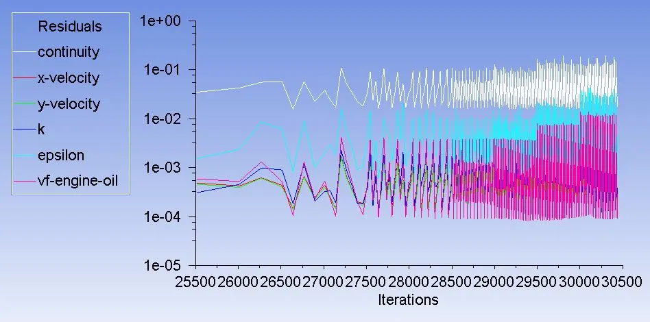
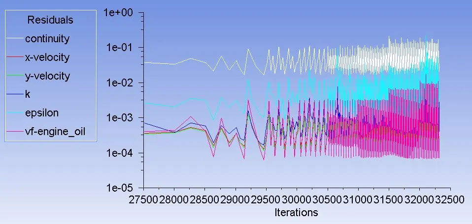
- Discuss the common errors that occurred in the simulation. A] 'Dynamic mesh failed' error. B] 'Negative cell volume detected' error.
PART I: Perform the four simulations in the Gearbox and then you have to compare the results among all the four cases.
In almost all industrial application, lubrication of moving component is necessary in order to minimise the friction between the moving component. In case of gearbox, the lubricant is kept in sump, as gears starts rotating the lubricant is carried to all teeths by sloshing mechanism. The objective of present study is to analyse the effect of sloshing on the lubrication of moving component.
Gear sloshing analysis is performed with two different lubricants namely Engine oil and n-Heptane liquid. Analysis is performed to check the lubrication of gear tooth with different lubricants and also analyse the sloshing phenomena in gearbox
.The figure below shows the 3D model of gearbox, but due to the limitation of Student version software we performed this simulation as 2D.
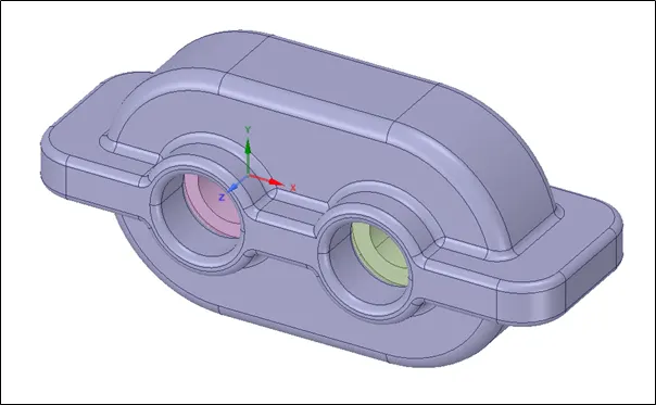
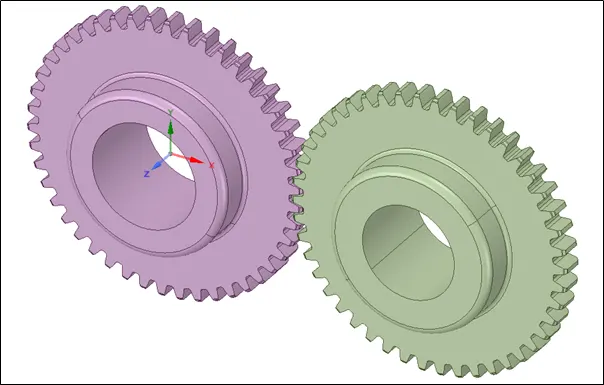
The gears inside the gearbox are the spur gears, as shown in the above figure. To study the flow behaviour of the lubricant we need to extract the fluid volume. The fluid volume is extracted as shown in figure below.
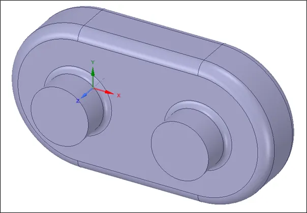
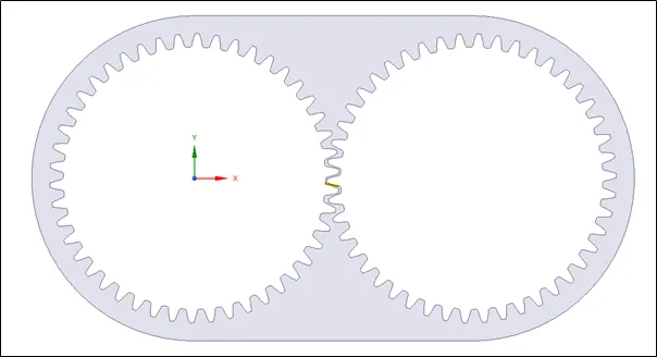
As we want to perform simulation over 2D geometry, we have to extract the 2D geometry from given 3D CAD model. To do so with the help of Split body tool we have cut the given 3D CAD model from middle plane. and copied the highlighted portion in another design window.
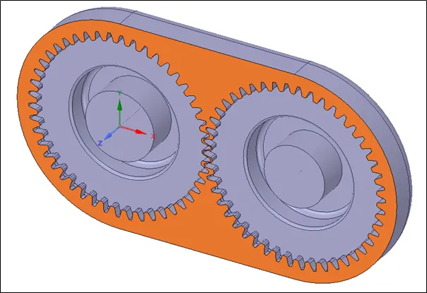
2D Geometry:
Meshing:
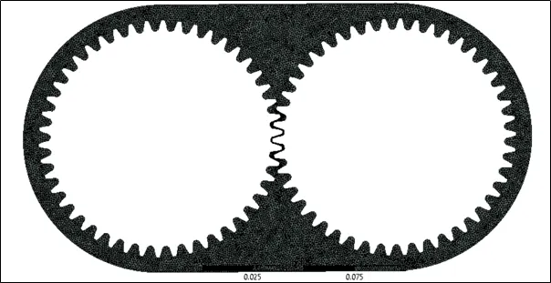
Element Size: 1 mm.
Number of elements: 20501
Number of Nodes:11388
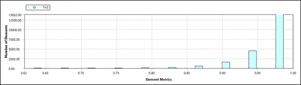
Element Quality:
Solver Settings:
Pressure based, Transient solver
Models:
Multiphase: VOF-->Implicit Model
Viscous: k-e-->reliazable-->Enhanced wall treatment
User Defined Function (UDF): The provided UDF is compiled with Visual Studio 2008. UDF code makes the both gears to rotate. The angular velocity of gears is taken as 200 rad/s in given program, hence the gears will rotate at the spped of 1910.82 RPM, which takes the 0.0314 sec.to complete one revolution of gear.
I have considered the 0.08478 sec. time for this analysis, which is approximately 2.7 revolution of gear.
Some reion of mesh is marked to define the level of the lubricant in sump.
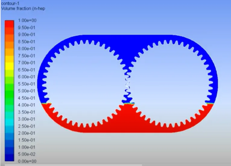
Dynamic mesh zones are enabled for right and left gears by defining their centers.
Left Gear: (0,0)
Right Gear: (0.115,0)
case1: 20% Immersion, Fluid - Engine oil
case2: 30% Immersion, Fluid - Engine oil
case3: 20% Immersion, Fluid - n-heptane
case4: 30% Immersion, Fluid - n-heptane
| Engine Oil | n-Heptane | |
| Density | 889 | 684 |
| Viscosity | 1.06 | 0.000409 |
Conclusion:
- Sloshing of n-Heptane is less than Engine oil, as the engine oil is more viscous than the n-Heptane.
- Being more viscous Engine oil has better sticking ability than n-Heptane and hence serve as better lubricant.
- With 30% immersion the lubricant spreads more uniformly than 20% immersion.
- Here in this case only 2.7 revolution of gear is considered for analysis due limitation of Student version of ANSYS Fluent, whereas this solution is not satisfacory for industrial use.
PART II:
DYNAMIC MESHING:
The dynamic mesh model can be used to model flows where the shape of the domain is changing with time due to motion on the domain boundaries. Combined with the six degrees of freedom (6 DOF) solver, dynamic mesh allows the trajectory of a moving object to be determined by the aero or hydrodynamic forces from the surrounding flow field.the dynamic mesh capability is used to simulate problems with boundary motion, such as check valves and store separations.The building blocks for dynamic mesh capabilities within ANSYS FLUENT are three dynamic mesh schemes, namely, smoothing, layering, and remeshing. A combination of these three schemes are used to tackle the most challenging dynamic mesh problems. However, for simple dynamic mesh problems involving linear boundary motion, the layering scheme is often sufficient. For example, flow around a check valve can be simulated using only the layering scheme.The motion can be a prescribed motion (e.g., you can specify the linear and angular velocities about the center of gravity of a solid body with time) or an unprescribed motion where the subsequent motion is determined based on the solution at the current time (e.g., the linear and angular velocities are calculated from the force balance on a solid body, which is what the six degree of freedom (6DOF) solver does .The update of the volume mesh is handled automatically by ANSYS FLUENT at each time step based on the new positions of the boundaries. To use the dynamic mesh model, you need to provide a starting volume mesh and the description of the motion of any moving zones in the model. ANSYS FLUENT allows you to describe the motion using either boundary profiles, user-defined functions (UDFs), or the Six Degree of Freedom solver (6DOF).
Smoothing
Nodes are moved as a spring and connectivity of nodes does not change. Smoothing is applicable to triangular and tetrahedral mesh. It can be used for hexahedral, quadrilateral and wedge shape elements.
Types
Spring based smoothing
Diffusion based smoothing
Spring Based Smoothing
Displacement of nodes generates the spring force which is given by:
ForceatNode=ΣKijnij⋅(Δxj-Δξ)">ForceatNode=ΣKijnij⋅(Δxj−Δξ)ForceatNode=ΣKijnij⋅(Δxj-Δξ)
Kij=KacΔxj−Δξ">Kij=KacΔxj−ΔξKij=KacΔxj−Δξ
where, Kac =Spring constant.
xi & xj are displacement of node i and its neighbor j.
At equilibrium, net force of connected springs at that node is zero.
Δξ=ΣKij∗ΔxjΣKij">Δξ=ΣKij∗ΔxjΣKijΔξ=ΣKij∗ΔxjΣKij
At convergence, ξ(n+1)=xn(i)+ξ(conver≥d).">ξ(n+1)=xn(i)+𐀀�ξ(conver≥d).ξ(n+1)=xn(i)+ξ(conver≥d).
where, n+1 and n denotes position of next time step and current time step.
Diffusion Smoothing
Equation of diffusion is given by, ∙=0">𐀀�∙𐀀�𐀀�𐀀�=0∙=0
where, 𝛾 is diffusion coefficient.
𝑢 is mesh displacement velocity.
=1">𐀀�=1𐀀�𐀀�=1
d is normalized boundary distance.
𝛼 is user input parameter.
Values of 𝛼 range from 0 to 2.
For diffusion smoothing, solution must be initialized. The dynamic mesh motion can be simulated afterwards.
x≠w=xold+u⋅Δt">x≠w=xold+u⋅Δtx≠w=xold+u⋅Δt
Parameters of Smoothing
Spring Constant Factor
Boundary Node Relaxation
Convergence Tolerance
No of Iterations
Diffusion Parameter
For the smoothing method, one can specify convergence tolerance and number of iterations depending upon experience. As number of iterations are completed during smoothing method, the mesh is updated. If the convergence tolerance is satisfied before the number of iterations, the dynamic mesh is updated to next time step.
Laplacian Smoothing:
It is simplest mesh smoothing method and most commonly used. It adjusts location of each mesh vertex at geometric center of neighboring vertices. Due to repositioning of vertices, it results poor quality elements. Hence, in FLUENT, repositioning is done only if there is possibility of improvement in skewness. It is applicable to the zone with triangular elements in 3D and linear elements in 2D.
Node position of x(m) is updated as:
ξm=Σxjmni">ξm=Σxjmniξm=Σxjmni
xim node position of node i at m iteration
xjm node position of neighboring node
ni no of neighboring node to i
Node position of x(m+1) is updated as
x(m+1)=ξm(1-β)+ξmβ">x(m+1)=ξm(1−β)+ξmβx(m+1)=ξm(1-β)+ξmβ
where, β is boundary node relaxation factor.
Layering:
It is applicable for 2D problems in case of linear motion.
Example: Piston moving inside the cylinder.
Addition/ deletation of cells at moving boundary is employed to maintain constant mesh.
Types of Layering:
Ratio Based Layering
Height based Layering
Split Factor and collapse factors are the factors that determine when layer of cell (hexahedral or wedge in 3D or quadrilateral in 2D) that is next to moving boundary is split or merged with adjacent cell layer respectively.
Parameters of Layering:
The Fig.shows the parameters for layering method.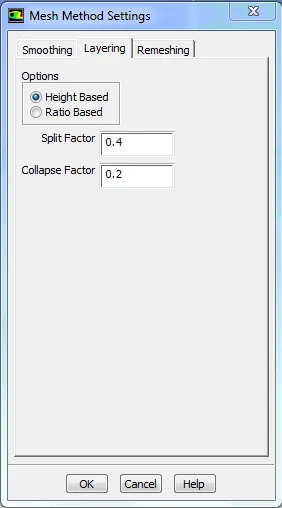
Remeshing:
This method can be applicable for large displacement problems. Node connectivity changes during remeshing. Further, this method is applicable for Triangular and Tetrahedral elements.
Cells/faces are remeshed only when the skewness and length scale exceeds specified values.
As Cells/faces are added/deleted, mesh connectivity changes.
Types of Remeshing Methods.
Local cell.
Local face
Remeshing Parameters
Region face
Example Region cell and Local face remeshing
Cutcell
2.5D
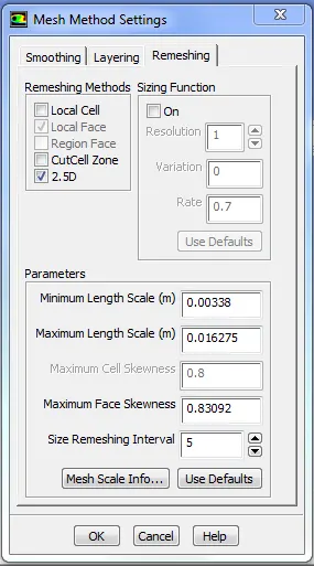
Remeshing Parameters:
Maximum length scale - It is maximum length scale in (m) shown in mesh scale information.
Minimum length scale - It is minimum length scale in (m) shown in mesh scale information.
Size Remesh Interval – It is the interval in which cells are marked for remeshing. The remeshing parameters are as shown in Fig.
Examples:
- Mixers and turbomachinery
-free surface flows
-flow of immiscible fluids
-sloshing problems
-fillling
FLUID SLOSHING EFFECT:
Fluid sloshing in fluid dynamics is considered as movement of liquid in another object. in order to study the slosh dynamics problem the liquid must have free surface. Where the liquid can interact with the container. The fluid waves are generated due to "inertial waves"
It is necessary to consider the sloshing of lubricant inside the gearbox casing in order to ensure proper lubrication of gear teeth. With this study one can wisely choose proper lubricant from the available solutions. It is also necessary to study dynamic forces and various design parameters.
The fluid sloshing effect can be good or bad. in some cases it is desirable have sloshing effect e.g. sloshing of lubricant in gearbox, mixing tanks. Whereas, in some cases sloshing is having adverse effects e.g. partially filled container on locomotive. it generates the additional hydrodynamic forces and impulsive pressure msy act on walls of container.
User Defined Functions (UDF):
UDF is standard C program which when dynamically loaded with ANSYS FLUENT enhances its standard feature. It is used to:
Customize boundary conditions, material property definitions, surface and volume reaction rates, source terms in ANSYS FLUENT transport equations, source terms in user-defined scalar (UDS) transport equations, diffusivity functions, and so on.
Adjust computed values on a once-per-iteration basis
Initialize solution.
Perform asynchronous (on demand) execution of a UDF
Execute at the end of an iteration
Enhance post processing
Improve existing ANSYS FLUENT models
Using UDF, we can customize ANSYS Fluent as per our requirement and increase its capability.
The DEFINE macros are provided in ANSYS FLUENT to define UDF, also uses some predefined functions to get the data from ANSYS FLUENT solver.
Commonly Encountered errors while performing simulation:
A] Dynamic mesh failed Error:
This problem comes as result of bad mesh quality. Due to bad mesh quality the remeshing is not done properly. and this error can be avoided using
- use triangular mesh in dynamic zone
- provide appropriate smoothing parameters
- And check time step size, distance moved in one time step must be less than the mesh size in dynamic zone
B] Negative cell volume detected' error.