Cyclone Separator Challenge

Aim:- To perform analysis on cyclone separator and calculate the separation efficiency and pressure drop.

Objective:-

To write a few words about any four empirical models used to calculate the cyclone separator efficiency.

To perform an analysis on a given cyclone separator model by varying the particle diameter from 1 μm to 5 μm and calculate the separation efficiency in each case. Discuss the results. [Use both the velocity's as 3m/sec.]

To perform an analysis on a given cyclone separator model by varying the particle velocity from 1 m/sec to 5 m/sec and calculate the separation efficiency and pressure drop in each case. Discuss the results. [Use particle diameter size as 5 μm for all cases & keep flow velocity same as particle velocity]

Empirical models used to calculate cyclone separator efficiency:

Li and Wang Model:

This model includes the particle bounce or re-entrainment and turbulent diffusion at the cyclone wall. The expression for particle distribution at the cyclone wall is obtained in 2D.

While developing this model following assumptions were made:

• Radial particle velocity and concentration profile are not constant for uncollected particles within the cyclone.
• Boundary conditions with the consideration of turbulent diffusion coefficient and particle bounce or re-entrainment on the cyclone wall are:

C = C₀ at θ = 0

`D_r ∂c/∂r=(1-α)ωc,` at r = D/2

• Tangential velocity is related to the radius of cyclone by: uRⁿ = Constant

The concentration distribution in cyclone is given as:

`c(r,θ)=(c_0 (r_w-r_n)exp{-λ[1/(K(1+n)) r^(1+n) ]})/(∫_(r_w)^(r_n)▒exp{1/(K(1+n)) r^(1+n) } dr)`

Where,

`K=((1-n)(ρ_p-ρ_g)d^2 Q)/(18μb(r_w^(1-n)-r_n^(1-n)))`

And

`λ= ((1-α)Kw_w)/(D_r r_w^n )`

The resultant expression of the collection efficiency for part of any size is given as

`η_i=1-exp⁡(-λθ_1)`

Where,

`θ_1=2π(S+L)/a`

Koch and Licht model:

This theory identifies the inherent turbulent nature of cyclone and distribution of gas, residence time within the cyclone. This model describes the particle motion at entrance and collection regions with the additional following assumptions:

• Tangential velocity of particle is equal to tangential velocity of gas flow i.e there is no slip in the tangential direction between the particles and the gas.
• The tangential velocity is related to the radius of cyclone by: uRⁿ = Constant.

Force balance and an equation on the particles collection yields the grade efficiency:

`ƞ_i=1-exp{-2[(Gτ_i Q)/D^3 (n+1)]^(0.5⁄(n+1)) }`

Where,

`G= (8k_c)/(k_a^2 k_b^2 )`

`n=1-{1-(12D)^0.14/2.5} 〖{(T+460)/530}〗^0.3`

`τ_i=(ρ_p d_pi^2)/18μ`

Iozia and Leith model (1990):

This model is modified version of Barth (1956) which is developed based on force balance. This model assumes that the particle carried by the vortex endures the influence of two forces, a centrifugal force and flow resistance.

The efficiency in terms of core length and core diameter are given as:

`η_i=1/(1+〖(d_pc⁄d_pi )〗^β )`

ẞ is an expression for slope parameter derived based on the statistical analysis of experimental data of cyclone with D = 0.25 m given as:

`β=0.62-0.87 ln⁡(d_pc⁄100)+5.21 ln⁡(ab⁄D^2 )+1.05[(ln⁡ab⁄D^2 )]^2`

And d_pc is the 50 % cut size given by Barth:

`d_pc=[9μQ/(πρ_c z_c v_(i max)^2 )]^0.5`

Where the core length zc and the core diameter dc are given as

`z_c=(H-S)-[(H-S)/((D/B)-1)][(d_c⁄B-1)] ,`, for d_c >B

`z_c=H-S` for d_c < B

`d_c=0.47D〖(ab/D^2 )〗^(-0.25) 〖(D_e/D)〗^1.4`

Lapple Model:

This model was developed based on force balance without considering the flow resistance. It is assumed that a particle entering the cyclone is evenly distributed across the opening. The particle that travels from inlet half width to the wall in the cyclone is collected with 50% efficiency. The semi-empirical model developed by Lapple to calculate 50% cut diameter d_pc is:

`d_pc=[9μb/(2πN_e v_i (ρ_p-ρ_g ) )]^0.5`

Where the Ne is the number of revolution

`N_e=1/a [h+(H-h)/2]`

The efficiency of collection of any size of particle is given by

`η_i=1/(1+〖(d_pc⁄d_pi )〗^2 )`

Simulation Methodology:

While modeling discrete phase modeling generally two phases come into picture i.e. continuous and discrete phase. Continuous phase is the fluid flowing in the control volume whereas the discrete phase is the particles interacting with the continuous phase. To simulate such phenomena DPM (Discrete Phase Modeling) model is used. Here in this model we can simulate by considering the interaction of particles with continuous phase or without considering interaction i.e. coupled and uncoupled flow of discrete particles.

Here in this study, we will perform simulation by considering two different cases,

• By varying the diameter of injected particles
• By varying the injection velocities.

Case		Name	Velocity (m/s)	Diameter (m)
Case_1		Case_1_1	3	1e-06
		Case_1_2		2e-06
		Case_1_3		3e-06
		Case_1_4		4e-06
		Case_1_5		5e-06
Case_2		Case_2_1	1	5e-6
		Case_2_2	2
		Case_2_3	3
		Case_2_4	4
		Case_2_5	5

Geometry:

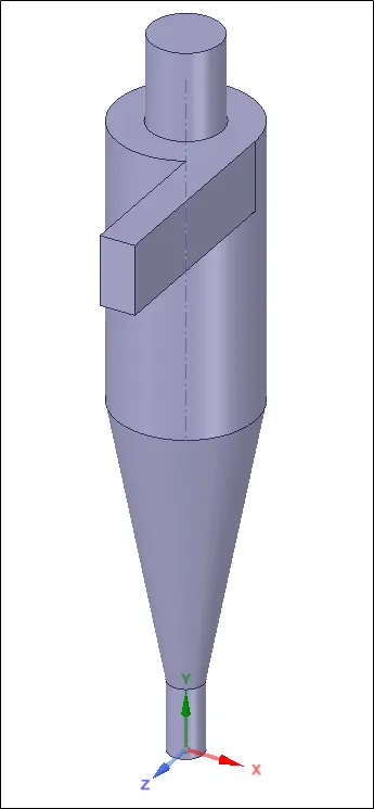
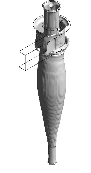
The cyclone separator geometry is in .stp format. Using Spaceclaim the fluid volume is extracted as shown in figure below.

Meshing:

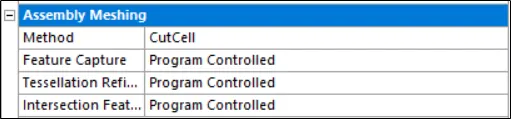
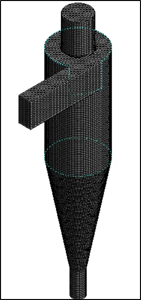
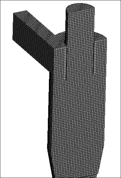
The unstructured mesh leads to more number of elements. So the hexahedral mesh is generated using Cut-shell approach of meshing available in workbench with default cell size.

The structural mesh gives the best results than unstructured mesh.

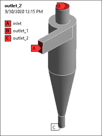
Named Selection:

To provide the appropriate boundary condition the name are given as shown below.

Case Setup:

Pressure based, steady state solver is used for simulation, with gravity enabled in negative Y direction.

g = - 9.81 m/s².

Viscous Model: K-e – RNG is model is used to account for the swirling effects generated due to flow. And for near wall treatment the Standard Wall Function is used.

DPM Model:

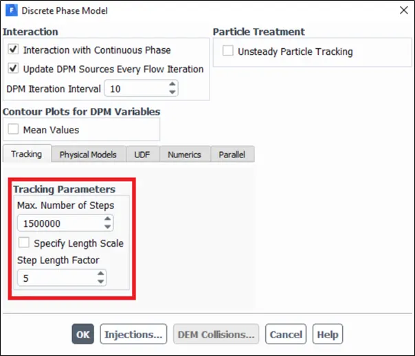
• “Interaction with the continuous phase” is enabled for solving equations in coupled manner.
• “Update DPM Sources At Every Flow Iteration” is enabled to calculate the particle source term every iteration.
• The maximum number of time steps to compute the trajectory of single particle. It is set to 1500000. In case fluent exceeds this time step, then it will automatically cancel to track that particle.

Particle Injection:

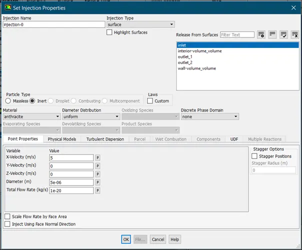
Injection type: Surface

Release from surface: Inlet

Particle type: Inert

Material: Anthracite

Flow Rate: 1e-20 kg/s

Boundary Conditions:-

Inlet and wall:- Reflect

Outlet(Top):- Escape

Outlet(Bottom/dustbin) – Trap

Reflect: rebounds the particle off the boundary with a change in its momentum as defined by the coefficient of restitution.

Escape: reports the particle as having “escaped” when it encounters the boundary. Trajectory calculations are terminated.

Trap: terminates the trajectory calculations and records the fate of the particle as “trapped”. In the case of evaporating droplets, their entire mass instantaneously passes into the vapor phase and enters the cell adjacent to the boundary.

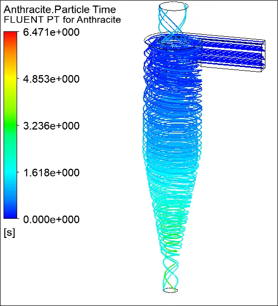
Case 1_1: Particle Diameter 1e-6 m.

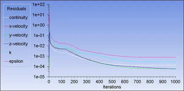
Residual:

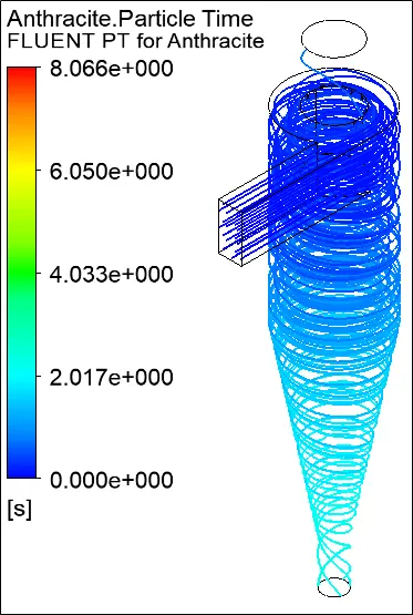
Anthracite particle time

Vortex core region:

Separator efficiency:

Efficiency = number of particles trapped/ number of particles tracked

= 18/120

=15%

Case 1_2: Particle Diameter 2e-6 m.

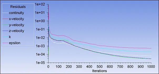
Residual:

Anthracite particle time:

Vortex core region:

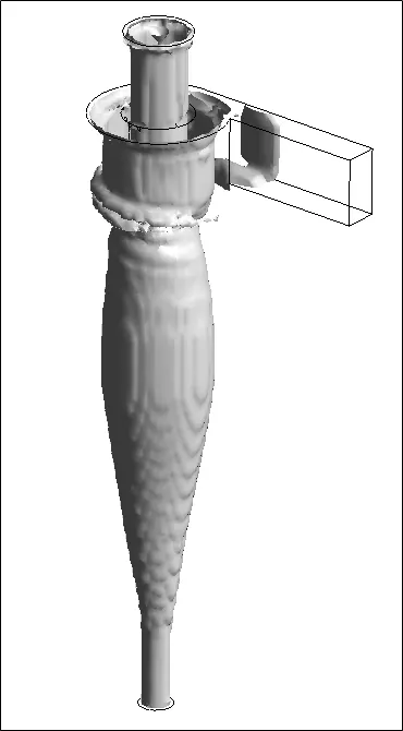
Separator efficiency:

Efficiency = number of particles trapped/ number of particles tracked

= 39/120

=32.5%

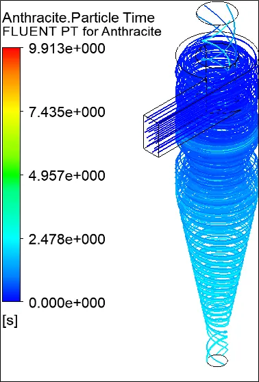
Case 1_3: Particle Diameter 3e-6 m

Residual

Anthracite particle time:

Vortex core region:

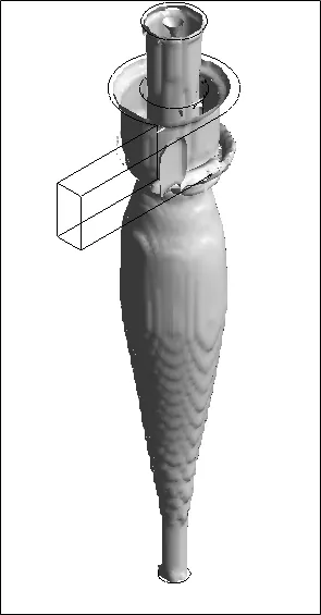
Separator efficiency:

Efficiency = number of particles trapped/ number of particles tracked

= 89/120

=74.16 %

Case 1_4: Particle Diameter 4e-06 m

Residual

Anthracite particle time:

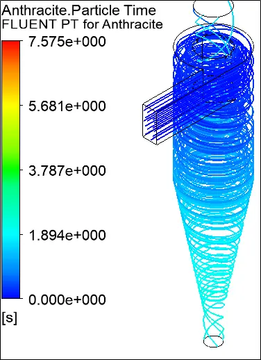
Cortex core region

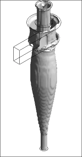
Separator efficiency:

Efficiency = number of particles trapped/ number of particles tracked

=88/120

=73.33%

Case 1_5: Particle Diameter 5e-06 m

Residual

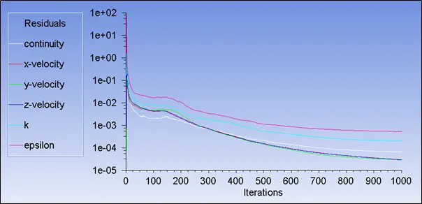
Anthracite particle time:

Vortex core region

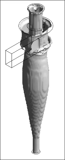
Separation Efficiency

Efficiency = number of particles trapped/ number of particles tracked

=111/120

=92.5 %

Pressure Drop:

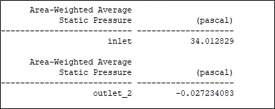
Pressure drop: 34.012829-(-0.027234083)

= 34.040063 Pa

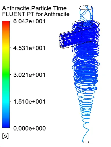
Case 2_1: Particle Velocity at inlet 1 m/s

Residual

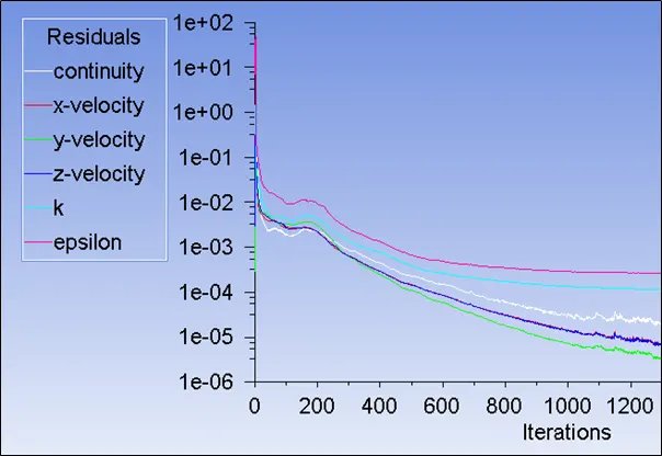
Anthracite particle time

Vortex core region

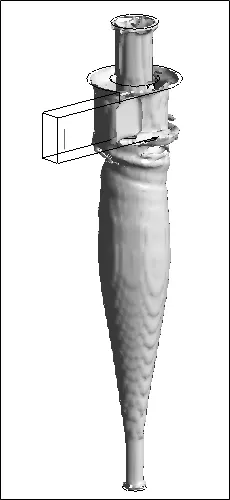
Separation Efficiency

Efficiency = number of particles trapped/ number of particles tracked

=4/120

=3.33 %

Pressure Drop:

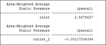
Pressure drop: 2.5675627-(-0.00017834394)

= 2.5677 Pa

Case 2_2: Particle Velocity at inlet 2 m/s

Residual

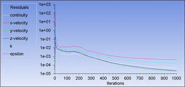
Anthracite particle time

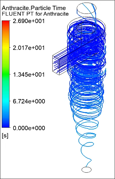
Vortex core region

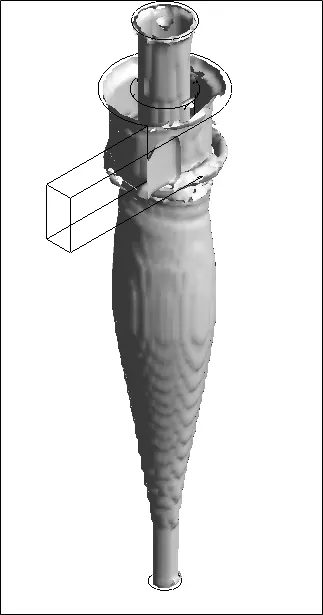
Separation efficiency:

Efficiency = number of particles trapped/ number of particles tracked

=12/120

=10 %

Pressure Drop:

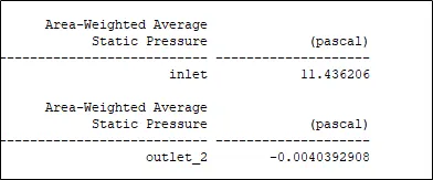
Pressure drop: 11.436206 – (-0.0040392908)

=11.4402 Pa

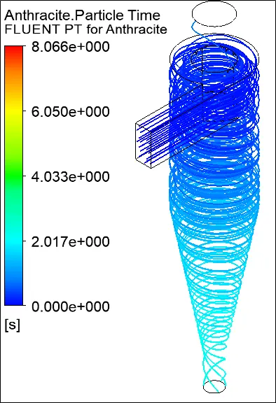
Case 2_3: Particle Velocity at inlet 3 m/s

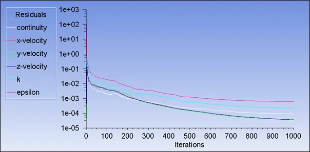
Residual

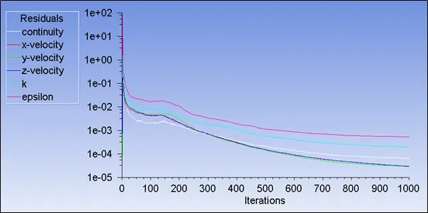
Anthracite particle time

Vortex core region

Separation Efficiency:

Efficiency = number of particles trapped/ number of particles tracked

=111/120

=92.5 %

Pressure Drop:

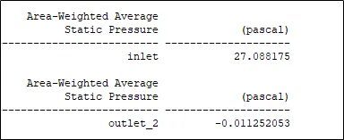
Pressure Drop: 27.088175-(-0.011252053)

=27.09942 Pa

Case 2_4: Particle Velocity at inlet 4 m/s

Residual

Anthracite particle time

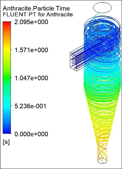
Vortex core region

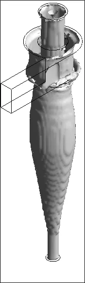
Separation Efficiency:

Efficiency = number of particles trapped/ number of particles tracked

=115/120

=95.83 %

Pressure Drop:

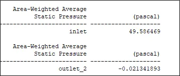
Pressure drop: 49.586469-(-0.021341893)

=49.6078 Pa

Case 2_5: Particle Velocity at inlet 5 m/s

Residual

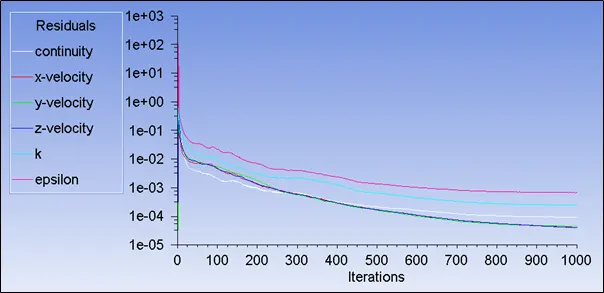
Anthracite particle time

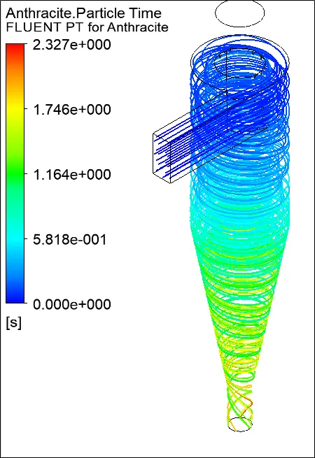
Separation Efficiency:

Efficiency = number of particles trapped/ number of particles tracked

=116/120

=96.66 %

Pressure Drop:

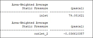
Pressure drop: 79.081621-(-0.036610357)

= 79.1182 Pa

Comparison:

Case_1:

Case	Particle Size (m)	Particle Velocity (m/s)	Particle Tracked	Particle Trapped	Particle Escaped	Separation Efficiency (%)	Pressure Drop (Pa)
Case_1_1	1e-06	3	120	18	49	15	34.040063
Case_1_2	2e-06		120	39	42	32.5
Case_1_3	3e-06		120	88	29	73.33
Case_1_4	4e-06		120	89	23	74.16
Case_1_5	5e-06		120	111	1	92.5

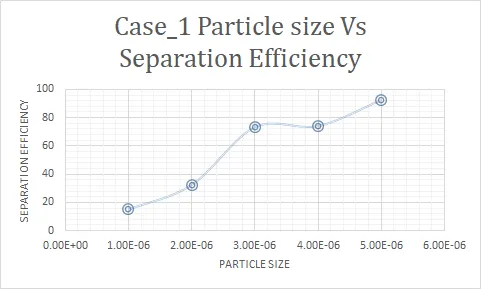
Variation of Separation Efficiency with the particle size.

Case_2:

Case	Particle Size (m)	Particle Velocity (m/s)	Particle Tracked	Particle Trapped	Particle Escaped	Separation Efficiency (%)	Pressure Drop (Pa)
Case_2_1	5e-06	1	120	4	34	3.33	2.5677
Case_2_2		2	120	12	17	10	11.4402
Case_2_3		3	120	111	1	92.5	27.09942
Case_2_4		4	120	115	5	95.83	49.6078
Case_2_5		5	120	116	4	96.66	79.1182

• It is observed from the table of case_1 that, as we increase the particle size the number of particles trapped also increases which leads to increase in separation efficiency.
• And as the particle velocity and inlet velocity are kept constant for Case_1, hence the pressure drop across the cyclone separator is constant.
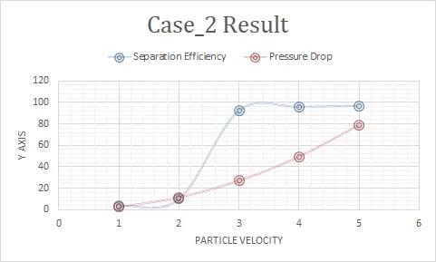
• Whereas, in Case_2 particle size is kept constant and the variation of separation efficiency with inlet velocity is studied.
• As the velocity is increased, by keeping the particle size constant also traps more particles, thereby increasing the separation efficiency.
• Also it can be observed from case_2 that, with increase in velocity the pressure drop also increases.
• With increasing value of particle diameter and velocity the time for which particle resides in cyclone separator decreases and hence the separation efficiency is improved.