Mixing efficiency

Aim: investigate the flow through mixing tee for fluid flow and heat transfer

Introduction:

The fluid streams mixing on tee are commonly encountered in piping system. To predict Heat transfer and mixing in tee joints is challenging using common CFD simulation and turbulence models. 

Theory:

The mixing of two streams of interesting normally which laeds to hydrodynamic disturbances and dislocations downstream the point of mixing. While redevelopment that will happen after mixing leads to decay of disturbances and that will affect the heat transfer as well. 

Importance in practical applications:

• Mixing of fluid at different temperature in T- joints in field of nuclear reactor safety. 
• Mixing of two air strams i.e. fresh outside air and recirculating air in air conditioning application. 
• Turbulent mixing in any type of plumbing works which intersects perpendicular to each other. 

Modeling approach:

We have two model of T-section one longer and one short. 

Pre-processing:

• Geometry:First of all we will import geometry using Spaceclaim. 

• Short Length Tee

• Meshing: to do meshing of given geometry I used ANSYS workbench. 

• Long Length Tee

Solver setting:

• Solver: Pressure based, Steady state
• Models:

Energy – On

Viscous – K-ℇ Realizable

• Materials:

Fluid: Air

• Boundary Conditions:

Inlet-x: velocity inlet

Inlet-y: velocity inlet

Outlet: pressure outlet

Wall: stationary wall, no slip condition

PV coupling scheme: SIMPLE

Results:

	Short MR 2	Short MR 4	Long MR 2	Long MR 4
No. of elements	12772	12772	15556	15556
Avg. outlet Temp.	30.255373	27.54817	30.30086	27.49567
No. of iterations till convergence	500	500	700	500

Model Dependence Study:

Sr. No.	Turbulence Model	Avg. Outlet Temperature	No. of iterations till convergence
1	K-ℇ Realizable	30.255373	500
2	K-ω SST	30.26164	1800

CASE 1: Short Length Tee

results shows the comparison of  cases with MR 2 and MR 4

Residuals:

• Mixing temperature at Outlet:

• Contour plots of velocity and pressure:

 

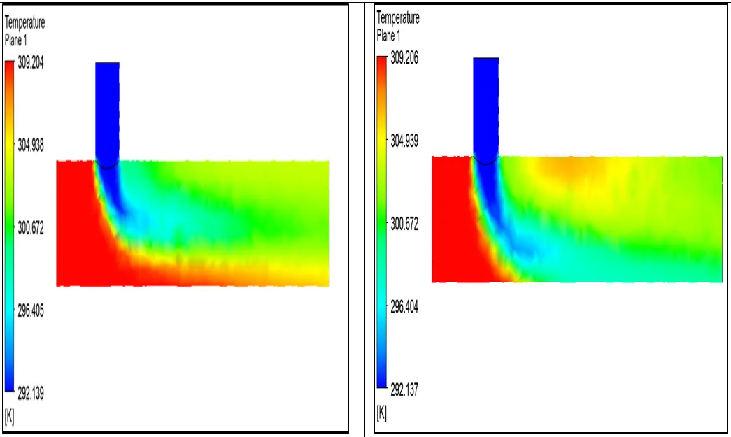
• streamline 

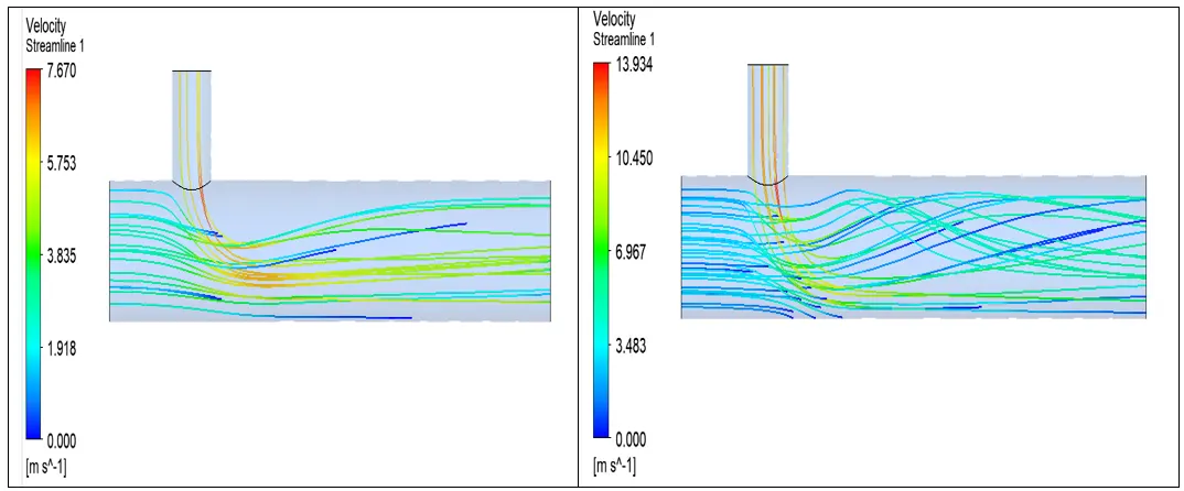
Case 2: Long Length Tee

• Residuals:

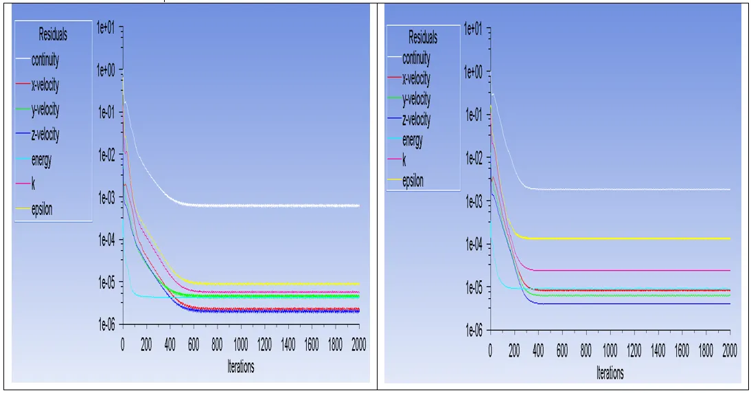
• Mixing temperature at Outlet:

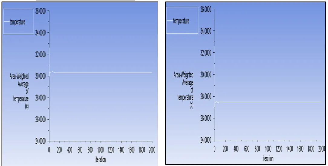
• Contour plots of velocity and pressure:

• stream line

Mesh Independence study:

Sr. No.	Element Size	Number of elements	Avg. Outlet Temperature	Number of iterations till convergence
1	Default	12772	30.255373	500
2	0.005 m	14251	30.23409	650
3	0.004 m	22159	30.29185	1700

Conclusion:

As we can see from the results presented above, it is observed that the solution is converged. the measure of effectiveness i.e. the standard deviation of temperature at outlet is near to 1. Hence, we can say that mixing is achieved nicely. Also, we have plot of area weighted average of temperature, that too with no variation as solution proceeds.

            In order to check the authenticity of solution, the simulation is done by changing certain parameters such as turbulence model, momentum ratio.

Where,

            Momentum ratio= (cold fluid velocity / hot fluid velocity)

And from this study it is observed that K-ℇ Realizable model predicts better mixing than K-ω SST model.

And while checking the effect of momentum ratio and length of pipe after joint on mixing efficiency, it is observed that increasing length after joint is not helping us to improve the mixing process but increasing the momentum ratio does. As the momentum ratio is doubled the standard deviation of temperature at outlet is decreased. And mixture temperature is decreased from 30.255373 to 27.54817.