Flow over a cylinder

Flow Over a Cylinder Simulation

using SolidWorks

BE (Mechanical Engineering)

by

Prajat Uday Sawant

Contents

Title

Introduction

Objective

Case Setup

Calculation

Observations

Conclusion

Introduction

SOLIDWORKS® Flow simulation is an intuitive computational Fluid Dynamics (CFD) Solution embedded within SOLIDWORKS 3D CAD that enables user to quickly and easily simulate liquid and get flows through and around your design.

Flow over a cylinder has the simple geometry and allows to understand complexities in the different flow patterns. Taking help of the Reynold’s number to understand flow over cylinder.

Reynold’s number is defined as the ratio of the inertial force to viscous forces within the fluid which are subjected to relative internal movement due to the different fluid velocities. The region where forces can change behaviour are boundary layer.

Laminar flow occurs at low Reynold’s number

Turbulent flow occurs at high Reynold’s number

Re= (rho*u*D)/mu

Where Re- Reynold’s Number

rho- Density of Fluid

u- Inlet Velocity

D- Diameter of Cylinder

mu- Dynamic Viscosity

Objective

The aim is to understand and simulate the transient flow over a cylinder in SolidWorks and observe the variation of velocity in a domain for Reynold Number.

Case setup

At the beginning of the simulation the part/model is required to be made. The horizontal cylinder is created of 0.02m in diameter and 0.05m in length in SolidWorks using tools and features as shown in figure Fig.1, then part/model (cylinder) is saved.

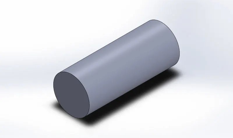
Fig.1

Firstly, baseline simulation has been observed Creating a new simulation giving the name of the project. For this project we chosen the analysis type as external, and physical features as Time-dependent (transient analysis). Under Time-dependent setting Total analysis time as 1 seconds and Output time step 0.1 seconds as per calculation further So that over a duration of simulation we get 10 outputs. The fluid is being taken as Air. Then the desired flow direction is being added, in this case the flow direction is add flow x-axis as shown in figure Fig.2. The velocity is taken as 1m/s.

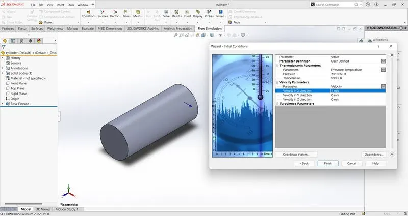
Fig.2

Immediately a computational domain is created as shown in Fig.3. in computational domain the fluid enters the domain, flow over a cylinder and will exit the domain in positive direction. Changed the domain and kept as 0.45m and also keeping the mesh size at 4. Run the simulation.

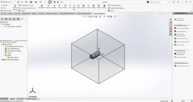
Fig.3

It taken few minutes for the calculations to complete. Add the cut plot of velocity at the centre of the cylinder and got the observations. Created an animation of the simulation. Fig. 4 show the velocity cut plot for baseline.

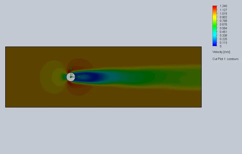
Fig.4

Similarly, to compare the simulation baseline Reynold’s number is increased by factor of 20%, 40% and 100%. And done same step to obtain the observations.

Calculations

Total simulation time being taken slightly more than the end time of the flow. Start time is calculated as (Total computational domain length/fluid velocity). The end time is calculated as 2 times the start time.

For baseline start time and end time

start time =0.45/1=0.45s

end time =2*0.45=0.9s

The fluid selected as Air which has the following properties:

rho=1.225 kg/m^3

mu=1.81*10^-5 kg/m.s

Taken diameter of cylinder as 0.02m

& Computational Domain Length as 0.45m

For Baseline Reynold’s number

For inlet velocity = 1m/s

Re=(rho*u*D)/mu=(1.225*1*0.02)/(1.81*10^-5)=1353

For increased 20%, 40% and 100% of Reynold’s number

	20%	40%	100%
Velocity(m/s)	1.12	1.4	2
Reynold's number	1623	1894	2706
Start time	0.4018	0.3214	0.225
End time	0.8036	0.6428	0.45

Observations

Case 1: For 20% increase in Reynold’s number, observed the blue shows the velocity is near to zero and also show the change its colour from blue to greenish-blue due to increasing in velocity. Red region shows the maximum velocity region. Shown in fig.5.

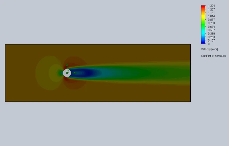
Fig.5

Case 2: For 40% increase in Reynold’s number, observed that the red region is lesser than in case 1. Rest contours are approximately the same as in case 1. Shown in fig.6.

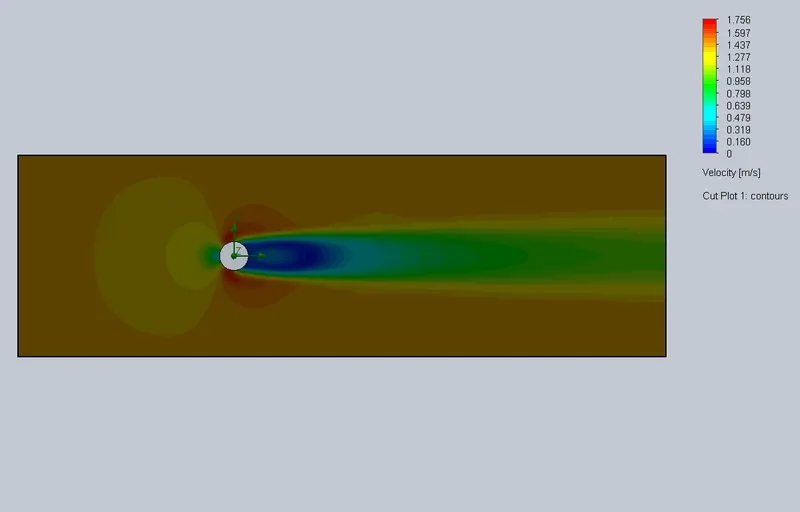
Fig.6

Case 3: For 100% increase in Reynold’s number, observed that the red region is lesser compared to previous two cases. Rest contours are approximately the same as previous cases. Shown in fig.7.

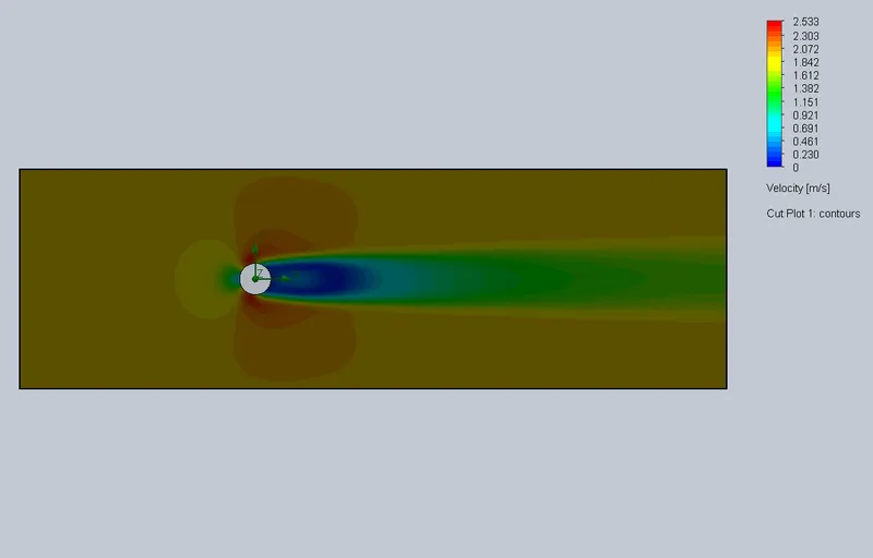
Fig.7

Conclusion

The basic concept of Flow over a cylinder simulation for different Reynold’s number using the SolidWorks were successfully studied by creating the horizontal cylinder and doing simulation for the baseline Reynold’s Number. And comparing with increased Reynold’s Numbers. For various increased in Reynold’s Number, it observed arbitrarily of the velocity are more or less the same.