Flow over a cylinder
FLOW SIMULATION OVER A CYLINDER USING SOLIDWORKS
Objective
To simulate flow over a cylinder (CFD Analysis) with an assumed initial Velocity for an External flow and running an Baseline Simulation and to make an parametric study with enhanced Reynolds Number.
Theory.
Computational fluid dynamics (CFD) is a branch of fluid mechanics that uses numerical analysis and data structures to analyze and solve problems that involve fluid flows. Computers are used to perform the calculations required to simulate the free-stream flow of the fluid, and the interaction of the fluid (liquids and gases) with surfaces defined by boundary conditions.
The Reynold's Number (Re) is defined as the ratio of Inertia force of a flowing fluid and the Viscous force. It is mathematically expressed as,
Re-(Inertia force/Viscous force) =( p V D/μ)
Where, p is mass density
V is average velocity of flow
D is diameter of pipe
μ is dynamic viscosity of flowing fluid
GEOMETRY
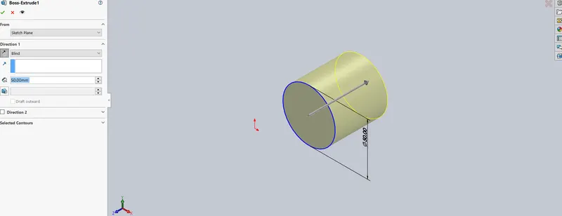
Diameter = 0.05m, Length=0.05m
Data
• Fluid - Air
• Temperature:- 293.2K (20 Deg celsius)
• Density of Air = 1.2041kg/m^3
• Initial Velocity=10m/s
Re= P.V.D/μ
** Dynamic viscosity...Ns/m^2 (also known as absolute viscosity) is the measurement of the fluid's internal resistance to flow while kinematic viscosity...m^2/s refers to the ratio of dynamic viscosity to density.
V.D Re
Kinematic Viscosity of Air @293K = 1.516*10^-5 m^2/s
CALCULATIONS
Re=[V.D]/v
[10 0.05]/1.516*10^-5
=32981
So, The 3 different inputs for Reynolds Numbers with diff factors are as follows,
Increased Factor Re Velocity
obtained 32981 10 (given)
+20% 39578 12
+40% 46173 14
+100% 65962 20
Procedure for Simulation
1. Create the Cylinder Model as per the data. 2. Select the Wizard and update the Parameters.
3. Analysis type :- External Flow with Time dependent (Transient analysis)
4. Select the Fluid as Air
5. In Initial ambient conditions set the velocity component along X-direction as 10m/s.
6. RUN the Flow Simulation
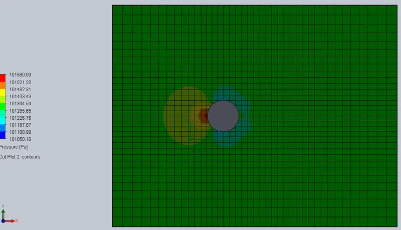
7. Insert the Cut Plots at the Centre for Plotting Velocity and Pressure Flows across the Cross Section.
8. Evaluate the obtained Results
9. Now Initiate an Parametric Study with different Reynolds Number ie;Initial Velocity.
10. Select Output Parameters as Cut Plots.
11. Create 3 Design Points for 3 different Initial Velocities.
12. Or the same can be done by creating new projects with different velocity inputs.
13. Evaluate the results with the obtained Plots.
Results
Cut Plots for Velocity
@10m/s
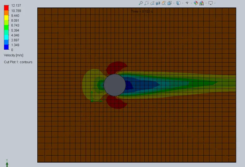
max velocity of 12.137m/s founded radially outward
@12m/s
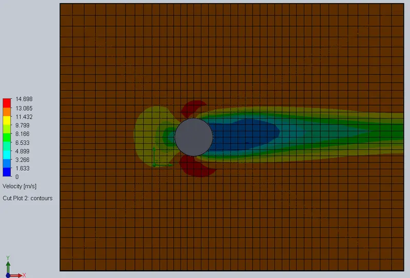
max velocity of 14.698m/s founded radially outward
@14m/s
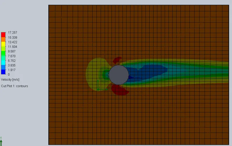
max velocity of 17.257m/s founded radially outward
@20m/s
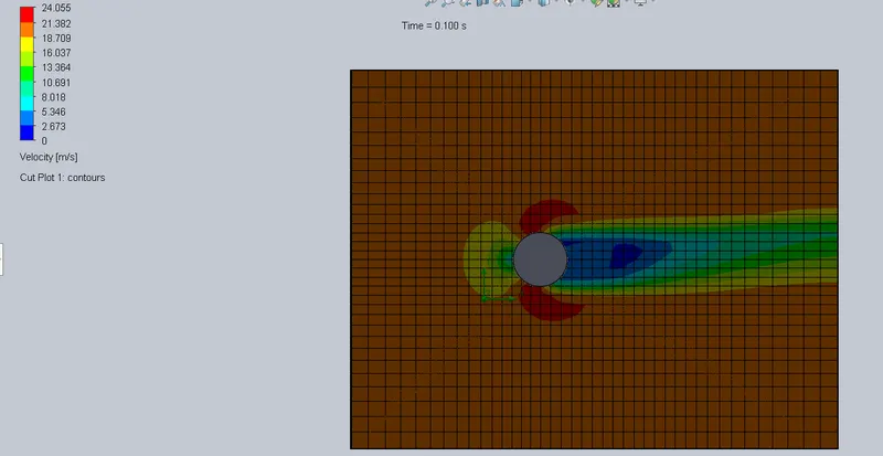
max velocity of 24.055m/s founded radially outward
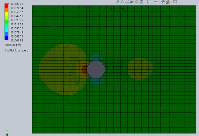
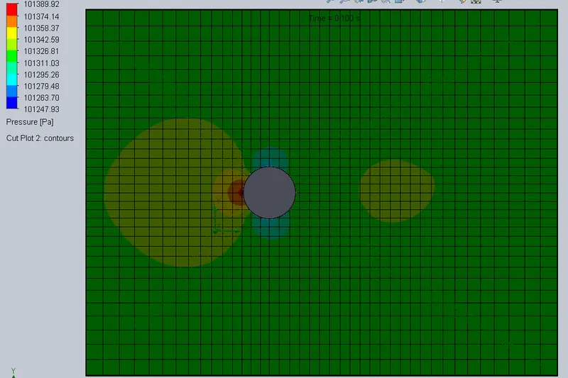
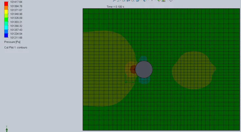
Cut Plot For Pressure
@10m/s
@12m/s
@14m/s
@20m/s
To Calculate Flow throgh Time
Initial Velocity for 4 cases are 10m/s, 12m/s, 14m/s & 20m/s.
To calculate flow through time for 4 different cases,
velocity [Distance/Time]
ie; Time [Distance/Velocity]
Case 1,
T=0.45/10 0.0455
Case2,
T=0.45/12 0.03755
Case3,
T=0.45/14 0.03215
Case4,
T 0.45/20 0.02255
Considering Buffer of 2x time for an Animation,
T1= 0,095
T2= 0.0755
T3= 0.06425
T4= 0.045s
Animation
@10m/s
Velocity Flow
Pressure Flow
@12m/s
Velocity Flow
Pressure Flow
@v=14m/s
Velocity Flow
Pressure Flow
@ V=20m/s
Pressure Flow
Observations
• A computational Domain is Created inside which an External flow over Cylinder is Performed.
• The Initial Flow is given only throgh X-direction.
• The presence of the Cylinder in the Domain acts as Obstruction to the flow.
• The entire domain is maintained in the applied Pressure/Velocity range whereas the region surrounding the Cylinder is affected which can be observed by the cutplots.
• Due to the cylindrical structure, there exists an Maximum Velocity region pointing radially outwards indicated by Red Colour in the Plots.
• The other side of the Cylinder towards exit of the flow experiences very low velocity range due to presence of obstruction indicated by Greenish Blue Colour in the Velocity Plots.
• With increase in the Reynolds Number, the inlet Velocity Increases and puts same effect on the walls of the Cylinder, only the extent of the Flow along with range of obstruction for the flow velocity changes.
• From the Pressure plots, kit can be observed that an Pressure is bulit up on the surface of the Cylinder facing the Inlet flow