External flow analysis over a circular cylinder

AIM

Simulate the flow over a cylinder and explain the phenomenon of Kármán Vortex Street using ANSYS Fluent.

PART-I:-

1. Simulate the flow with the steady and unsteady case and calculate the Strouhal Number for Re= 100.

PART-II:-

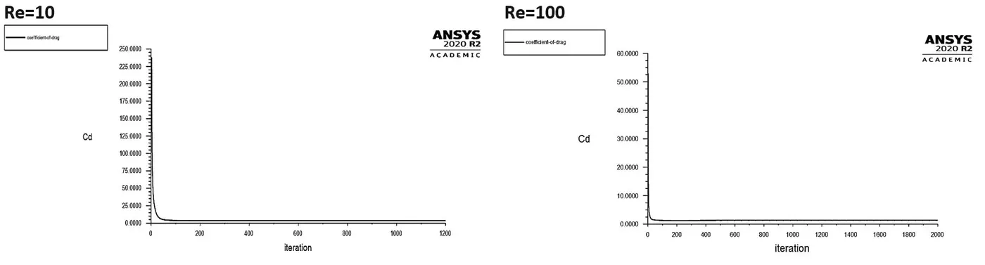
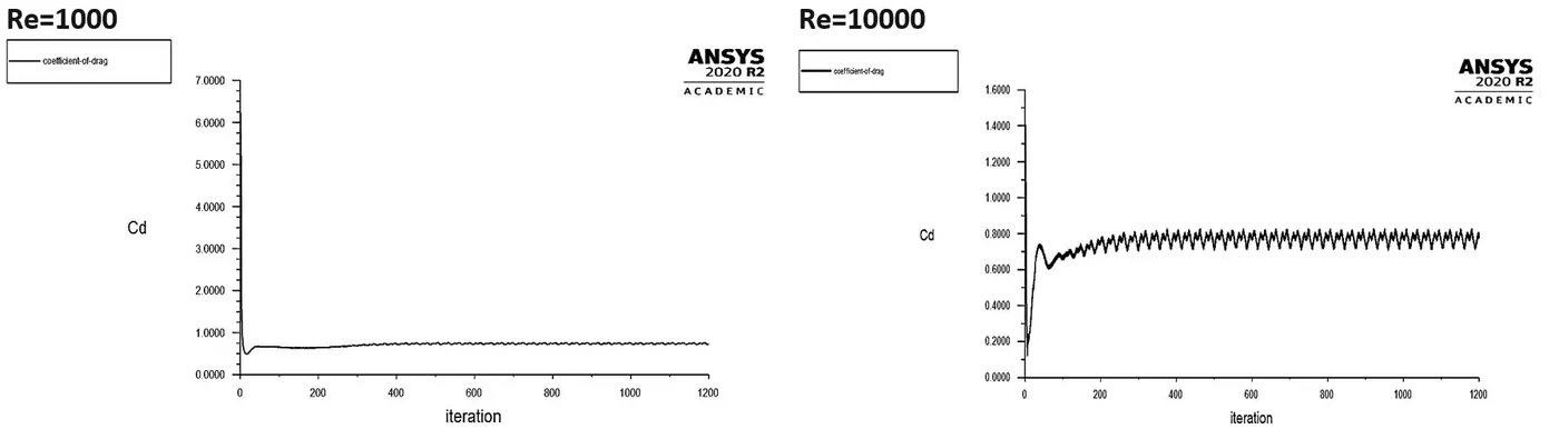
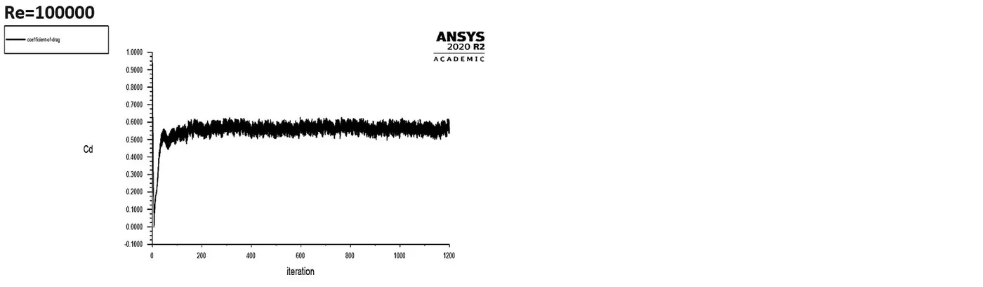
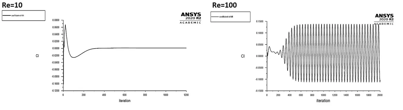
1. Calculate the coefficient of drag and lift over a cylinder by setting the Reynolds number to 10,100,1000,10000 & 100000. (Run with steady solver)
2. Discuss the effect of Reynolds number on the coefficient of drag. [we should validate Results with any standard literature and error should be within 5 %]

Expected results:-

1. In both approaches, show that the flow has converged. What quantities or plots need to be looked at determining that the flow has converged?
2. Plots of the coefficient of drag and lift.
3. Plots to show vortex shedding behind the cylinder.
4. Mention the preferred material at the end of the challenge submission page.

THEORY

For very small value of Re, the flow completely remains laminar around the cylinder with no recirculation and no instability. For larger values of Re, a regular pattern of alternating vortices are generated and these eddies are unstable and successively leave the cylinder to propagate in the wake, to form the so called Von Karman vortex street. These vortices produce a sinusoidal force acting on the body perpendicular to the flow.

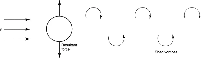
Vortex shedding

As a fluid particle flows toward the leading edge of a cylinder, the pressure on the particle rises from the free stream pressure to the stagnation pressure. The high fluid pressure near the leading edge impels flow about the cylinder as boundary layers develop about both sides. As a fluid particle flows toward the leading edge of a cylinder, the pressure on the particle rises from the free stream pressure to the stagnation pressure. The high fluid pressure near the leading edge impels flow about the cylinder as boundary layers develop about both sides. Since the innermost portion of the shear layers, which is in contact with the cylinder, moves much more slowly than the outermost portion of the shear layers, which is in contact with the free flow, the shear layers roll into the near wake where they fold on each other and coalesce into discrete swirling vortices. A regular pattern of vortices called a vortex street trail aft in the wake. Von Karman vortices form at all scales of fluid motion. A vortex street will form only at a certain range of flow velocities, specified by a range of Reynolds numbers (Re), typically above a limiting Re value of about 90.

For a cylinder, the frequency ω (in Hz) of the shedding is related to the diameter D(m) and wind speed v (ms⁻¹) via the Strouhal number S such that S = ωD / v.

PHYSICS OF THE PROBLEM

The problem encompasses a circular cylinder with a diameter of D=2m submerged in a stream with an undisturbed speed of V = 1 m/s (for our first part of the project), whereas for the second part of our project inlet velocity varies according to the different Reynolds numbers. The problem statement is shown in the below figure.

For this problem, there is no easy analytical solution to describe the behavior of the fluid (except for potential flow, which is an ideal case).

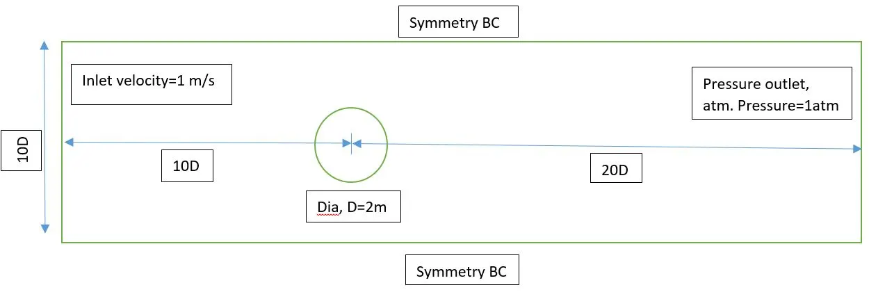
The behavior of the flow around a circular cylinder is very complex and highly dependent on the Reynolds number. The boundary layer in laminar regimes detaches at an angle of `theta = 82^0` because of the existence of an adverse pressure gradient. Due to the symmetry of the cylinder, a curious phenomenon appears named von Karman street, consisting of alternate vortices emitted by the cylinder. The vortices are detached periodically, and it directly relates their frequency to the Strouhal number.

PRE-PROCESSING, MODELING AND SOLVING APPROACH

Meshing:

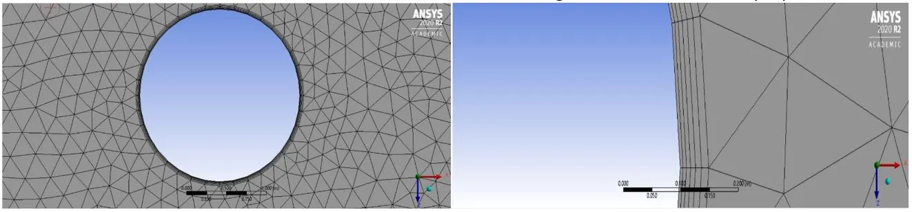
We use ANSYS inbuilt Meshing tool for the discretization of our flow domain for solving. For this project; we want our mesh to be triangular dominant, and we’ll use a few more important refinements to simulate the flow behavior correctly. The mesh for the study of the cylinder will not be uniform. Some areas of the domain need to contain a higher cell density (mainly the walls of the cylinder and its prolongation).

NOTE: On the walls and downstream of the cylinder it is necessary to have a highly refined mesh. It will allow the user to compute the drag coefficient and to observe the von Karman street both with high accuracy. However, if the simulation is too much time-consuming or it is done with a Reynolds number such that no vortices are generated, it is recommended to reduce the refinement of the mesh.

Adding method: Select the body and after selecting the body; in the method section just select the triangles. Now our mesh is triangular.

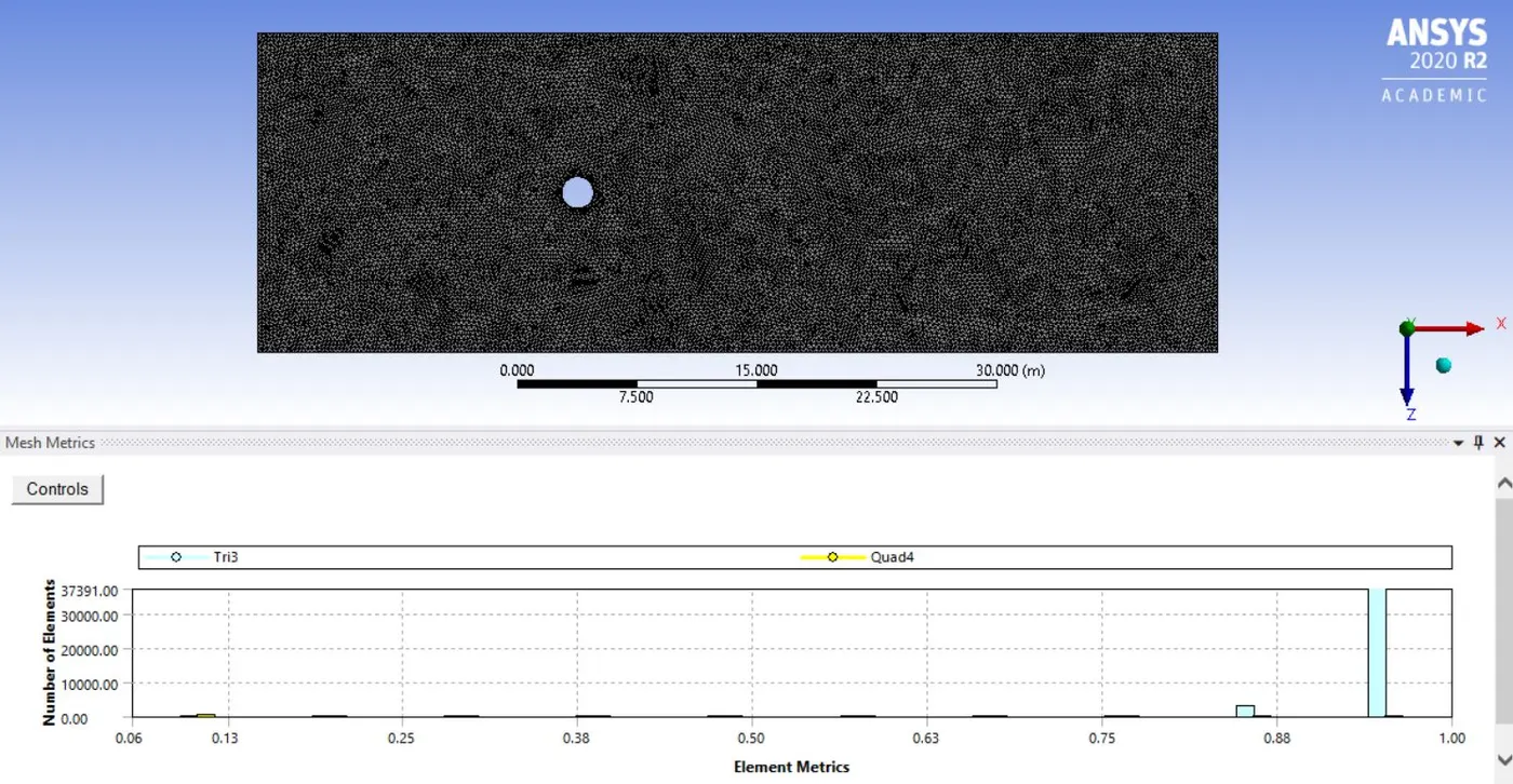
Element Size: Choosing element size is totally based on user experience. Here for this simulation, we’re using our element size to be 0.25m. For element size=0.25m, we’re getting a number of nodes=41534 and a number of elements=40642. Our element size is perfect and no need to decrease the element size more, because it does not make much difference in the solution, and if we decrease the element size below the 0.25m, it eventually increases the simulation time.

Sizing: With our default mesh, we can see after zooming to the circle it is looking more like a polygon (with maybe 12 or 13 faces). So, it’s not perfect and to be honest, we can never get a perfect circle unless we have an infinite number of edges. However, if we see our default mesh, we can notice that there are sharp corners that can affect the flow field. So, one thing we want to do in CFD is to make sure that our geometry–on top of which we are going to simulate the flow–is captured perfectly.

Case 1:

• For both steady and transient problem and for the given Re number of 100, set the properties of the user-defined material such as density to 1 kg/m3 and viscosity to 0.02 Pa-s.
• Assign the proper boundary conditions such as inlet velocity as 1 m/s, outlet pressure as 1 bar (atmospheric) and rest default.
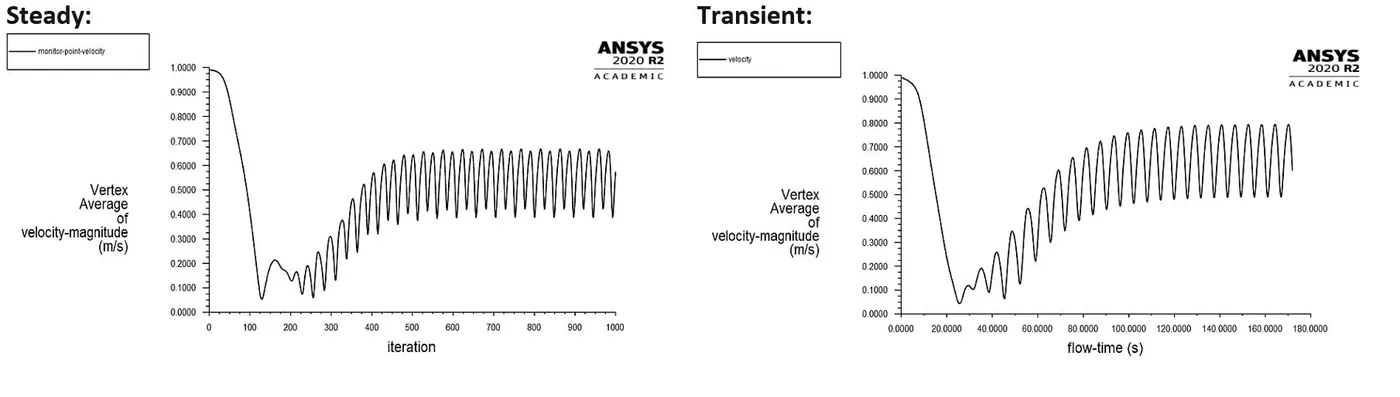
• Create a monitor-point at a distance of 8m from the centre of the cylinder at which velocity plot has to be generated.
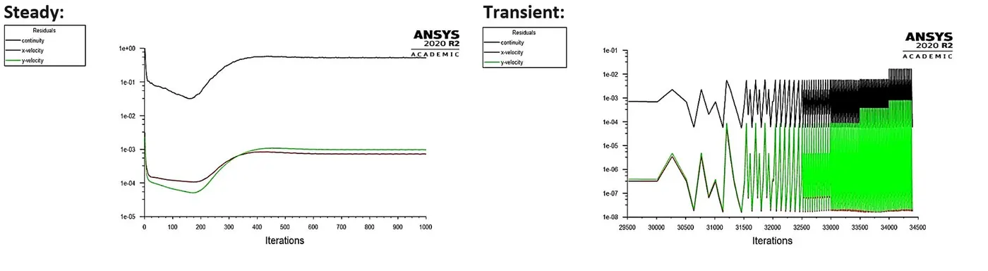
• Run the calculations for n number of iterations and carefully observe the residual plot to check if the solution has converged. Also observe velocity contour plot for vortex shedding.

Case 2:

• Now to get a Reynold's number of 10,100,1000,10000, we need to change the velocity and thus i have set the properties of air as follows : viscosity = 0.01 Pa-s, density = 1 kg/m3, velocity = 5.05e+10 and absolute pressure = 1 bar.
• Similarly vary the velocity to achieve the Reynold's number of 100000.
• Define the drag and lift so as to compute the coefficient of drag and lift respectively.

RESULTS :

PART-I:

Here we are comparing the results obtained from the two different setups, i.e. steady-state and transient. The aim behind doing that is to get an idea of using a steady-state or transient solver for a particular problem.

Residuals Plot:

Plot for Vertex average of Velocity:

Velocity Contour:

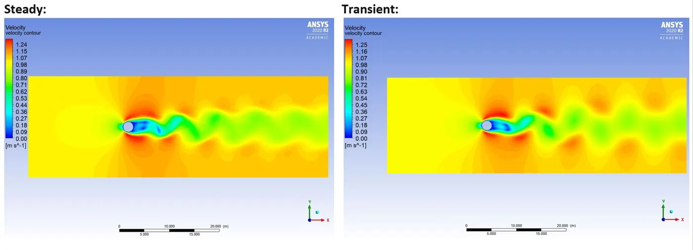
Steady-state simulations are typically performed to get conclusive answers. So, any intermediary solution that we get is not time accurate. Suppose, at 250 iterations, we get a particular value of velocity, then this value of velocity does not co-relate to a particular time. And this is all because of which we are not getting accurate results. We have seen vortex shedding but anyway we can’t calculate the frequency parameter–the vortex frequency–and that too Strouhal number. That’s why we need a Transient simulation.

In Transient simulation, we solve equations w.r.t. time. So at every time step, we solve equations accurately, meaning we can trust that results. Since it does the calculation for each time-steps, hence we can calculate the Strouhal number in this case.

PART-II:

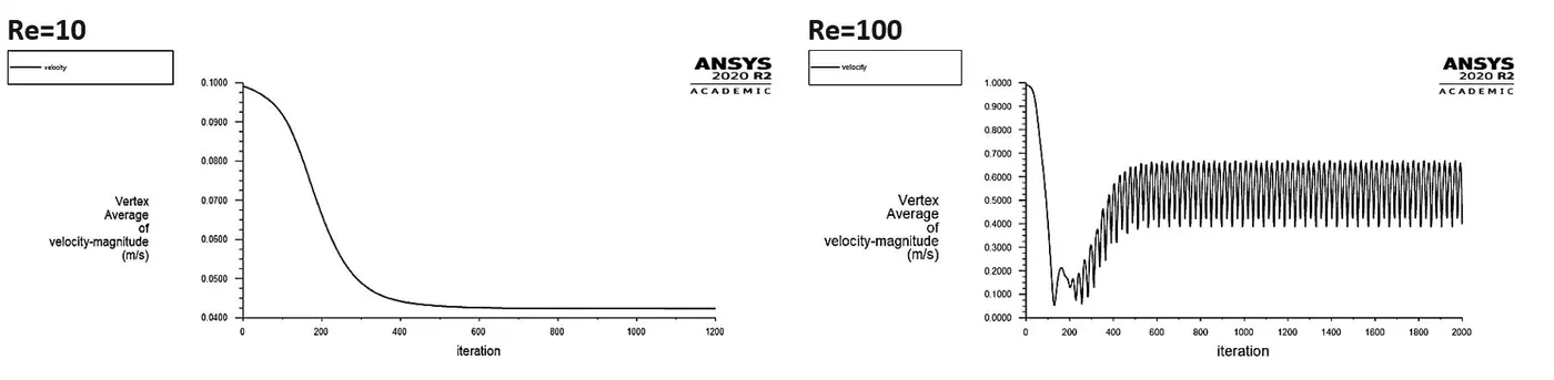
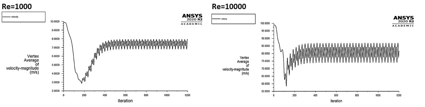
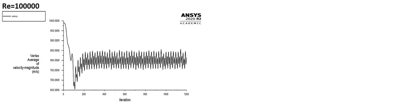
Plots for Vertex average of velocity:

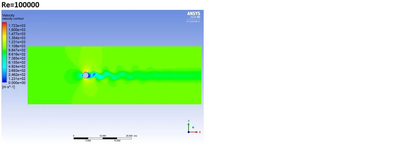
Velocity Contours:

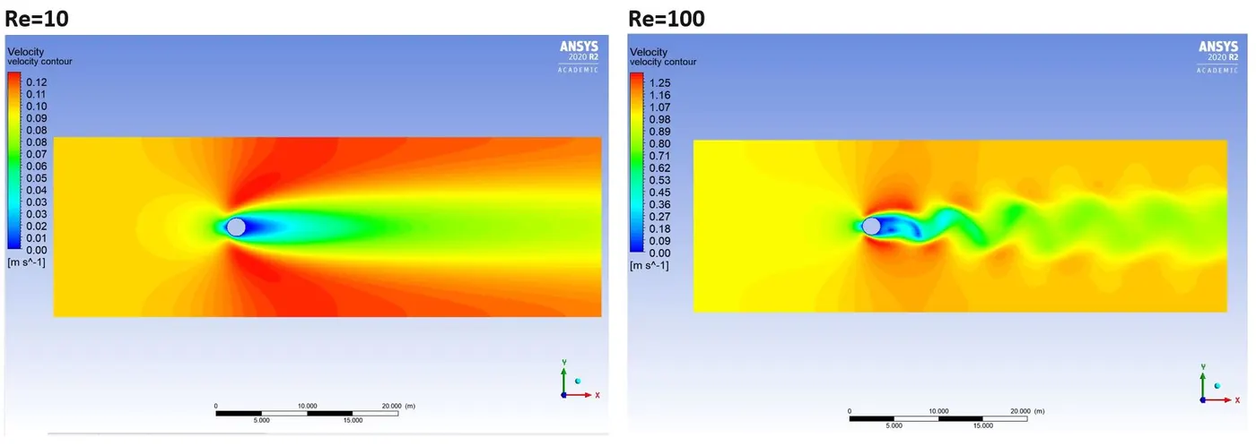
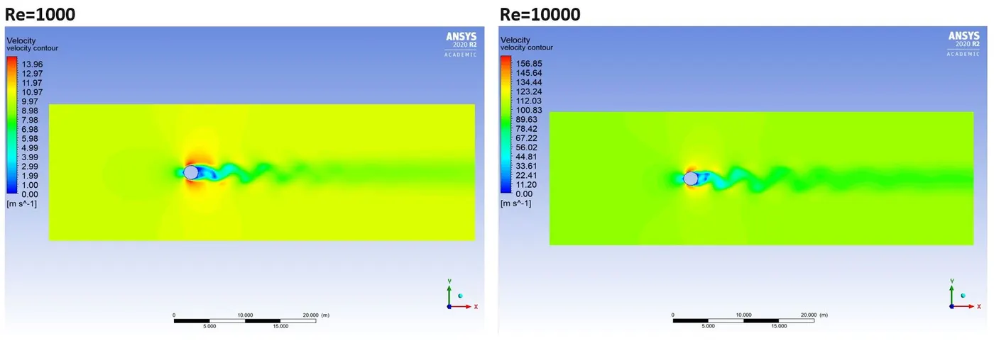
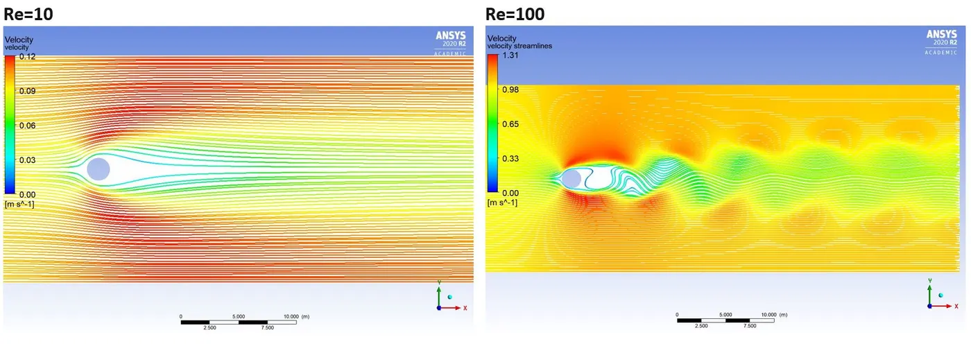
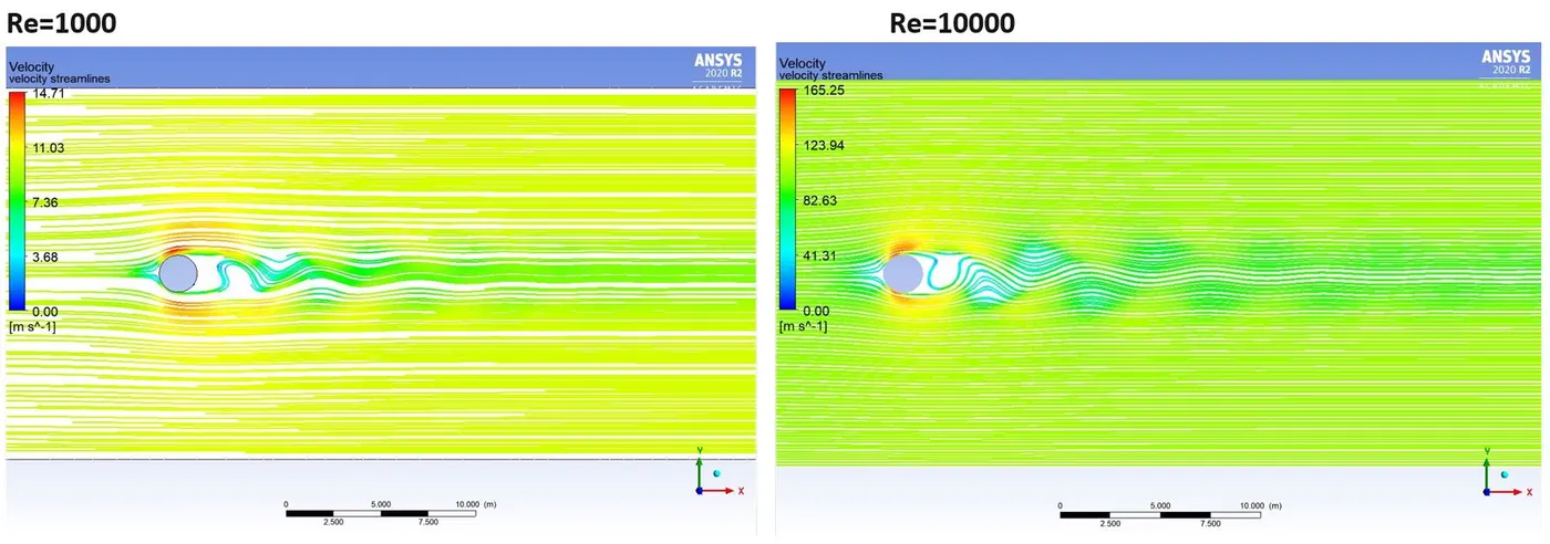
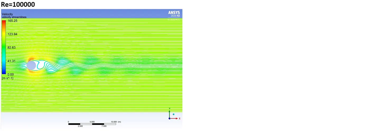
Velocity Streamlines:

Coefficient of drag plot:

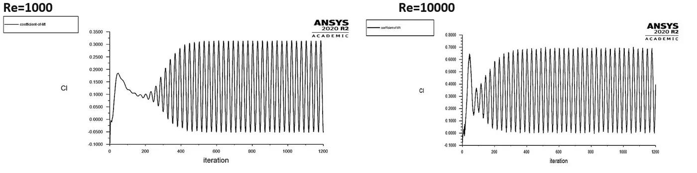
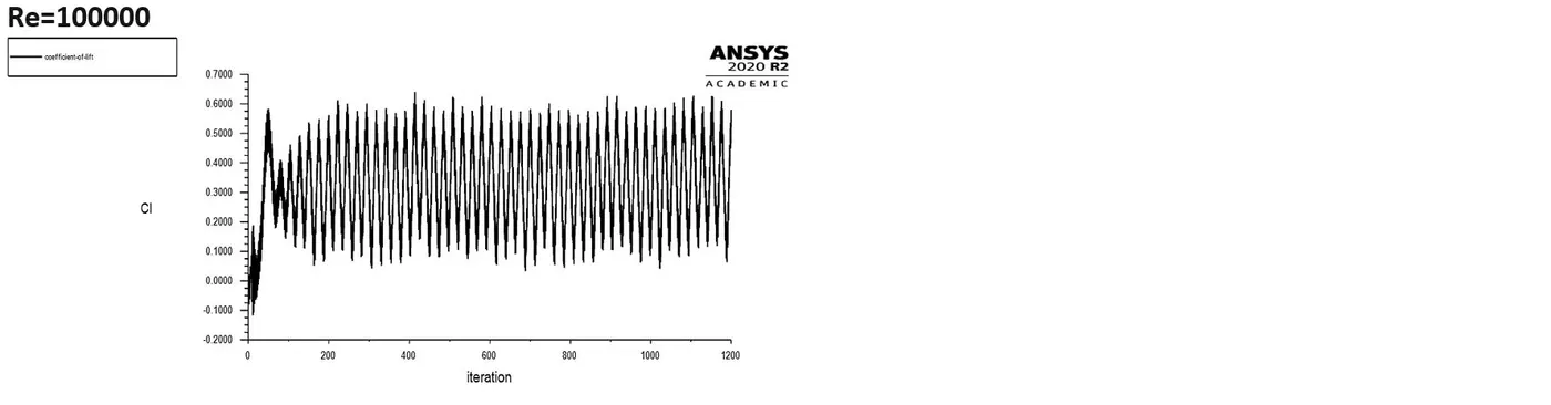
Coefficient of lift plot:

CONCLUSION

The wake structure behind the circular cylinder has been computed for two-dimensional flow using second order accurate implicit finite volume Navier–Stokes solver SIMPLE. Computations have been carried out for Reynold's numbers between 5.5 and 10,100,1000,10000 covering three different characteristic regimes creeping flow (L1), steady closed near wake (L2) and the laminar vortex shedding regime(L3). By increasing the Reynold's number beyond the critical value i.e., above 47, one can notice that the inertial forces start to dominate over viscous forces. The coefficient of drag (Cd) starts decreasing and there is a significant fluctuation in the Coefficient of lift (Cl) and the Vertex average of Velocity magnitude at the monitoring point rises at the same time. From the table we can notice that as we increase the Reynolds number, our Drag coefficient is decreasing whereas the Lift coefficient increasing. When we compare these results with the findings of Rajani et al. [2], we find that our results agree reasonably well.

REFERENCE PAPER : Numerical simulation of laminar flow past a circular cylinder by B.N.Rajani, Sekhar Majumdar and A. Kandasamy.