Fitting a curve to predict values of specific heat upon varying temperatures and find linear fit, cubic fit and splitwise method
AIM : To write a code to fit a linear and cubic polynomial and compare it with real time data , to find the best fit , also to use splitwise method to obtain a best fit.
THEORY: Curve fitting is widely used in examination of relationship between dependent and independent variables, used in regression models , calculation of errors, this helps us determine the best method to find which polynomial is suited to predict data within a range( interpolating) or outside of a range (extrapolating). They are very powerful to determine the trend in a scatter plot. If scattered data is deviating beyond a permissible range ,it can be concluded that it is not a good fit.
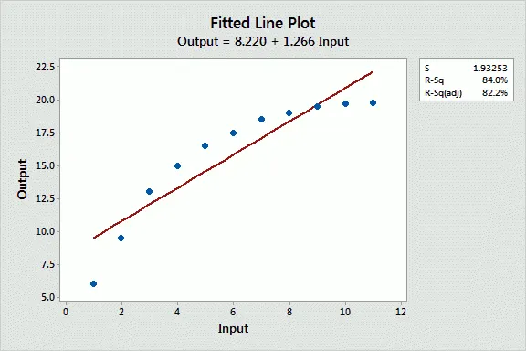
We are often required to find the best fit rather than perfect fit.
Best fit: It offers the best approximation of a given trend of scattered plot i.e. the error is at a minimum and best describes the trend.
Perfect fit: It is more accurate and follows the exact trend of scattered data with nearly zero error at a given dataset but often leads to exaggerated results beyond a data range when the degree of polynomial increases.(it fits exactly)
WAYS TO GET:
1.Perfect fit: Increasing the degree of polynomial, using splitwise method, but increasing the degree leads to bad conditioning without proper precautions.
2.Best fit: Least sum of squares i.e.R^2 should be equal to 1.
3.Improved cubic fit: Using splitwise the deviation can be reduced to a great extent.
In some scenarios linear fit is best fit compared to cubic fit considering extrapolation.
FINAL CODE INCLUDING LINEAR,CUBIC & SPLITWISE METHOD:
clear all
close all
clc

% load data
cp_data = load('data');
temp = cp_data(:,1);% access data in first column
cp = cp_data(:,2); % access data in second column

% plot graph from data points
plot(temp,cp,'linewidth',4)
grid on
xlabel('TEMP[K]')
ylabel('Specific heat[Kj/Kmol-K]')

% curve fit

% for linear variation let cp = aT + b

co_effs = polyfit(temp,cp,1); % gives coefficient of given data based on equation

predict_cp = polyval(co_effs,temp);% to find predicted values of cp

% for cubic variation let cp = aT^3 + bT^2+ cT+d

[co_effs1,s,mu] = polyfit(temp,cp,3) % gives coefficient of given data based on equation with mean

predict_cp2 = polyval(co_effs1,temp,s,mu);% to find predicted values of cp


%goodness of fit

e = predict_cp2-cp;%calculate error
sse = sum(e.^2); % sum of squares of errors
ssr = sum((cp-mean(cp)).^2); % sum of squares due to regression element operation
sst = ssr + sse; % total sum of squares
r_square = (ssr/sst);

if r_square > 0.95
    display('good fit');

else
    display('bad fit');

end

% splitwise method used to fit a curve based on a range divided to datasets

temp1 = cp_data(1:500,1);
cp1 = cp_data(1:500,2);

temp2 = cp_data(500:1000,1);
cp2 = cp_data(500:1000,2);

temp3 = cp_data(1000:1500,1);
cp3 = cp_data(1000:1500,2);

temp4 = cp_data(1500:2000,1);
cp4 = cp_data(1500:2000,2);

temp5 = cp_data(2000:2500,1);
cp5 = cp_data(2000:2500,2);

temp6 = cp_data(2500:3000,1);
cp6 = cp_data(2500:3000,2);

temp7 = cp_data(3000:3200,1);
cp7 = cp_data(3000:3200,2);

% finding coefficients for splitwise

[co_eff1,s1,mu1] = polyfit(temp1,cp1,3);
predicted_cp1 = polyval(co_eff1,temp1,s1,mu1);

[co_eff2,s2,mu2] = polyfit(temp2,cp2,3);
predicted_cp2 = polyval(co_eff2,temp2,s2,mu2);

[co_eff3,s3,mu3] = polyfit(temp3,cp3,3);
predicted_cp3 = polyval(co_eff3,temp3,s3,mu3);

[co_eff4,s4,mu4] = polyfit(temp4,cp4,3);
predicted_cp4 = polyval(co_eff4,temp4,s4,mu4);

[co_eff5,s5,mu5] = polyfit(temp5,cp5,3);
predicted_cp5 = polyval(co_eff5,temp5,s5,mu5);

[co_eff6,s6,mu6] = polyfit(temp6,cp6,3);
predicted_cp6 = polyval(co_eff6,temp6,s6,mu6);

[co_eff7,s7,mu7] = polyfit(temp7,cp7,3);
predicted_cp7 = polyval(co_eff7,temp7,s7,mu7);

% to compare curve fit
hold on
plot(temp,predict_cp,'linewidth',2,'color','r');% linear fit
plot(temp,predict_cp2,'linewidth',2,'color','g');% cubic fit

plot(temp1,predicted_cp1,'linewidth',1,'color','y');% for splitwise method
plot(temp2,predicted_cp2,'linewidth',1,'color','y');
plot(temp3,predicted_cp3,'linewidth',1,'color','y');
plot(temp4,predicted_cp4,'linewidth',1,'color','y');
plot(temp5,predicted_cp5,'linewidth',1,'color','y');
plot(temp6,predicted_cp6,'linewidth',1,'color','y');
plot(temp7,predicted_cp7,'linewidth',1,'color','y');
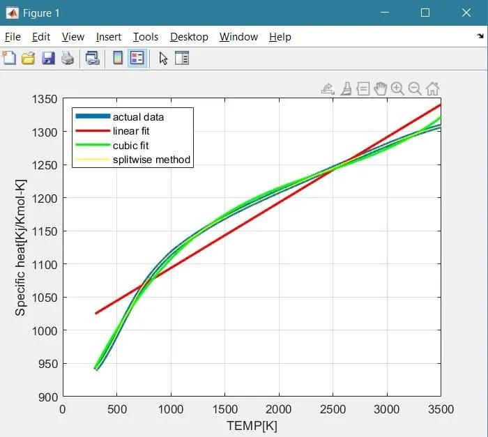
legend ('actual data','linear fit','cubic fit','splitwise method','location','northwest');
An obtained graph which helps understand Linear,cubic,splitwise fits and their relation with original data:
THE FOLLOWING METHODS ARE USED TO EVALUATE GOODNESS OF FIT:
1.R-Squared (R²):
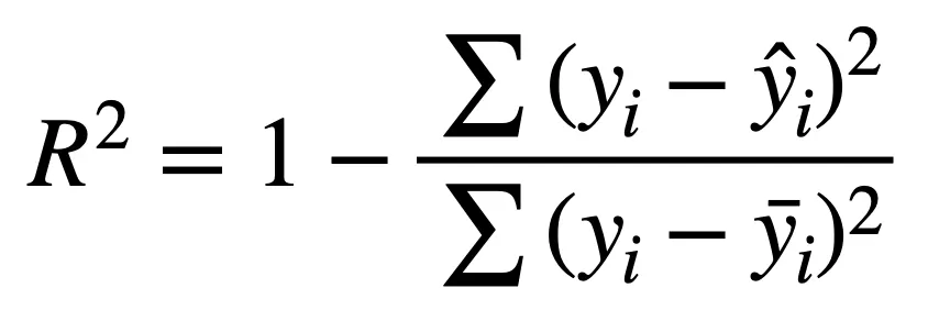 [y = dependent variable values, y_hat = predicted values from model, y_bar = the mean of y]
The R² value, also known as coefficient of determination, tells us how much the predicted data, denoted by y_hat, explains the actual data, denoted by y. In other words, it represents the strength of the fit, however it does not say anything about the model itself — it does not tell you if the model is good, whether the data you’ve chosen is biased, or even if you’ve chosen the correct modelling method¹. I will show this using examples below.
The R² value ranges from 0 to 1, with higher values denoting a strong fit, and lower values denoting a weak fit. Typically, it’s agreed that:
R² < 0.5 → Weak fit
0.5 ≤ R² ≤ 0.8 → Moderate fit
R² > 0.8 → Strong fit.
2.Adjusted R² (Adj. R²):
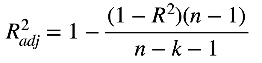 [n = the number of data points in the sample, k = includes the number of variables in the model, excluding the constant term (the intercept).]
The adjusted R² improves upon the R² by giving insight into whether a model’s R² value is because of how good the fit is, or rather because of it’s complexity.
3.Mean Absolute Error (MAE)
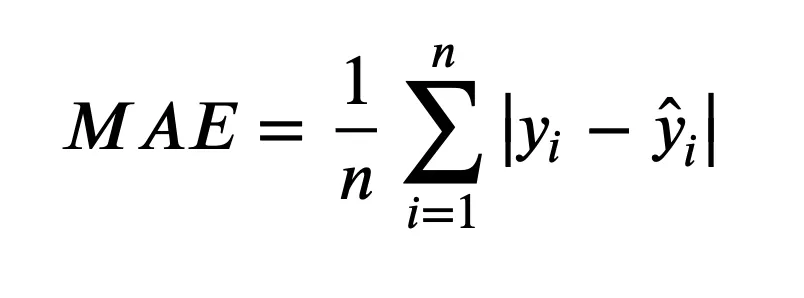 [n = number of points, y = actual point, y_hat = predicted point]
The MAE is the sum of all the error magnitudes divided by the number of points, so essentially the average error.
Therefore, the lower the MAE, the less error in your model.
4.Mean Squared Error (MSE)
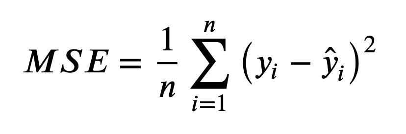 [n = number of points, y = actual point, y_hat = predicted point]
The MSE is the sum of the squares of all errors divided by the number of points. Note that, since in each instance the error is actually squared, it cannot be directly compared to the MAE, because it will always be of a higher order.
Thus, as with MAE, the lower the MSE, the less error in the model.
5.Root Mean Squared Error (RMSE)
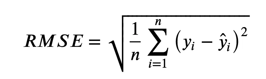 [n = number of points, y = actual point, y_hat = predicted point]
RMSE is the square root of the MSE. This is in a way a more useful metric, and now since both MAE and RMSE have the same ‘order’ of error, they can be compared with each other.
As with both MAE and MSE, lower MSAE → lower error.
Explanation for linear and cubic fit:
1.Linear fit: we use (co_effs = polyfit(temp,cp,1)) to fit the curve for linear fit and plot the graphs after finding the coefficients using (predict_cp = polyval(co_effs,temp))
2.cubic fit: we use ([co_effs1,s,mu] = polyfit(temp,cp,3)) to fit a cubic curve with structure and mean and repeat the same procedure as we did for linear fit
Explanation of splitwise method
After loading the data from a given file the data is divided to seven sets of data which varies with temperature.
Then each predicted cp for a range of temperatures is found out using polyval command along with their own 'mu','s' values and then the graph is plotted
RESOURCES:
Skill-lync projects
http://mrpaynemath.weebly.com/uploads/3/8/9/9/38994693/math3201ch5.3notes-workings.pdf
(Note: Considering scenarios where the code is to be long, the linear, cubic fit and splitwise method has been included in the same code ,but the learnings and intended results do not change. No errors were made)