Writing a code to solve an otto cycle and plot p-v diagram

Aim: To create a code that can carry out the following functions in matlab,

a.)Plot p-v diagram for an otto cycle.

b.)Find the thermal efficiency of the cycle.

Theory and code:

The otto cycle comprises of four processes

a.)Reversible Adiabatic compression.

b.)Isochoric heat addition.

c.)Reversible adiabatic expansion.

d.)Isochoric heat rejection.

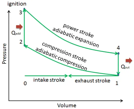
assumptions made,

gamma = 1.4

t3=2500K

p1=101325 pa

Terms used in the code:(governing equations)

1.)Compression Ratio (cr): it is the ratio of volume before compression and volume after compression.

`cr = (vs+vc)/(vc)`

where, vs= swept volume, vc = clearance volume

`v1=(vs+vc)`

`v2=vc`

`cr=(v1)/(v2)`

also,

`cr=(v4)/(v3)`

2. State variables:

They include properties like pressure , temperature and volume, which help to determine work done, heat added, which will be useful in calculation of thermal efficiency

At state 1, p=101325 pa, t=300K ,

bore = 0.1
stroke = 0.1
con_rod = 0.15
cr = 10

`vs=pi/4*(d)^2*l`where 'd' denotes diameter of bore

`vc=(vs)/(cr-1)`

At state 2 being reversible adiabatic compression,

`p2 = p1*cr^gamma`(assume gamma to be 1.4 for air)

`t2 = (p2*v2*t1)/(p1*v1)`(using charles law)

At state 3 being isochoric heat addition,

v2=v3

`p3 = (p2*t3)/(t2)`(assume t3=2500k)

At state 4 being reversible adiabatic expansion,

v4=v1

`p4 = (p3)/(cr^gamma)`

using this input we can plot the graph and find thermal efficiency but when we plot we get a graph like below which is an error in graph if coded as follows

plot([V1 V2 V3 V4 V1],[P1 P2 P3 P4 P1], ‘color’,’r’)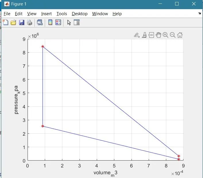

This is where we use a function where the variation of volume based on the angle is calculated and called in the main program,

Another key point is both main program and function should be in the same directory in the path of matlab to be able to call the function,

else the following error shows up,

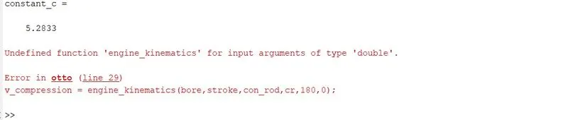
another error is while we create an array we forget to use element operator .

Also we need to be careful while using variable we want to find and interchange them

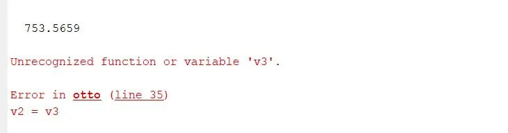
after correcting such errors and using funtion to call the volume values the code goes as follows, and we make sure that name of function and saved file is same

`V/(Vc) = 1+ 0.5(cr-1)* [ R+1 -cos(theta) — (R² -sin²(theta)⁰.5]`

(to find variation of volume with crank angle.)

the dimensions include (bore,stroke,length of connecting rod, starting crank angle,ending crank angle), which can be then used in finding volume at different crank angles. we use linspace command to space he intervals equally for a smooth curve.

function [v]= piston_kinematics(bore,stroke,con_rod,cr,start_crank,end_crank)
bore = 0.1;
stroke = 0.1;
con_rod = 0.15;
cr = 10;
a = stroke/2
r= con_rod/a
v_s = (pi/4)*bore^2*stroke
v_c = v_s/(cr-1)

crank_angle = linspace(start_crank,end_crank,100);

% formula
t1 = 0.5*(cr-1);
t2 = r+1-cosd(crank_angle);
t3 = (r^2-sind(crank_angle).^2).^0.5;

v = (1+t1*(t2-t3)).*v_c;

end

the final matlab program is as follows;

clear all
close all
clc

% inputs
gamma = 1.4
t3 = 2500

% state variables
p1 = 101325
t1 = 300

% engine geometric parameters
bore = 0.1;
stroke = 0.1;
con_rod = 0.15;
cr = 10;

% swept and clearance volume calculation
v_swept = (pi/4)*bore^2*stroke;
v_clearance = v_swept/(cr-1);

v1 = v_swept + v_clearance
v2 = v_clearance

% state 2 variables to find pressure
p2 = p1*cr^gamma
constant_c = p1*v1^gamma
v_compression = piston_kinematics(bore,stroke,con_rod,cr,180,0);
p_compression = constant_c./(v_compression.^gamma);

t2 = p2*v2*t1/(p1*v1)

% state variables at 3
v3 = v2
p3 = p2*t3/t2
constant_c = p3*v3^gamma;
v_expansion = piston_kinematics(bore,stroke,con_rod,cr,180,0);
p_expansion = constant_c./(v_expansion.^gamma);
% state varaible at 4
v4=v1

p4 = p3/(cr^gamma)

% thermal efficiency
thermal_efficiency = (1-1/(cr^gamma))*100

% graphs 
hold on
grid on
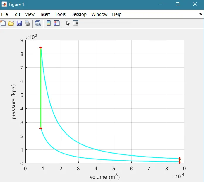
plot (v_compression,p_compression,'linewidth',1.5,'color','c')
plot (v_expansion,p_expansion,'linewidth',1.5,'color','c')
plot ([v2 v3],[p2 p3],'linewidth',1.5,'color','g')
plot ([v4 v1],[p4 p1],'linewidth',1.5,'color','g')
plot (v1,p1,'*','color','r')
plot (v2,p2,'*','color','r')
plot (v3,p3,'*','color','r')
plot (v4,p4,'*','color','r')
xlabel('volume_ (m^3)')
ylabel('pressure_ (kpa)')
 

hold on command prevents previous line plots from getting removed,

grid on command spaces the intervals equally

plot helps in generating graphs.

the final outputs are as follows.

gamma =

    1.4000


t3 =

        2500


p1 =

      101325


t1 =

   300


v1 =

   8.7266e-04


v2 =

   8.7266e-05


p2 =

   2.5452e+06


constant_c =

    5.2833


a =

    0.0500


r =

    3.0000


v_s =

   7.8540e-04


v_c =

   8.7266e-05


t2 =

  753.5659


v3 =

   8.7266e-05


p3 =

     8443750


a =

    0.0500


r =

    3.0000


v_s =

   7.8540e-04


v_c =

   8.7266e-05


v4 =

   8.7266e-04


p4 =

   3.3615e+05


thermal_efficiency =

   96.0189

p-v diagram