Final Project: Electric Rickshaw modelling

Electric Rickshaw modelling

Theory:

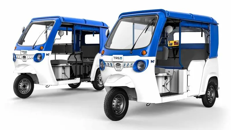
An electric rickshaw or e-rickshaws is a vehicle that has 3 wheels, with two in the rear and one in the front powered by one electric motor. These are eco-friendly and has low fuel cost. They are mostly manufactured in India and China. The most common types of motor used are Permanent Magnet Synchronous Motor (PMSM). One of the popular E-rickshaw model in India , the Mahindra Treo is shown below,

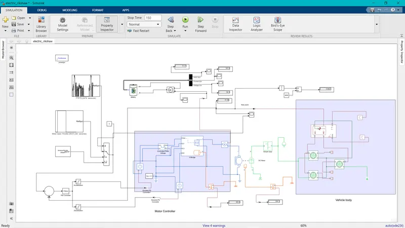
The simulink model of electric Rickshaw is shown below

Simulink model:

starting with drive cycle :

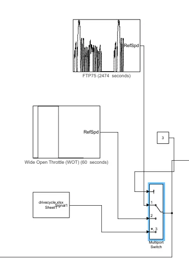
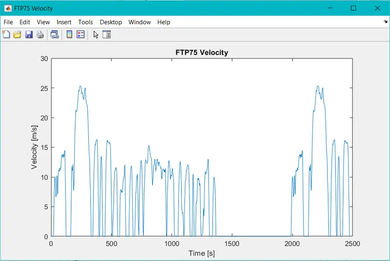
Here I have given Three Different Drive cycles as input which is used to test the vehicle performances. These drive cycle will have high speed, low speed, braking conditions in it. There are different drive cycles like WOT, FTP75 etc., Here in this model I have used FTP 75, WOT Manually prepared in excel Drive Cycle source

Plot of FTP75 drive cycle

Plot of WOT drive cycle

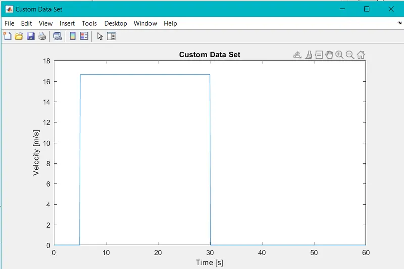
Spread sheet Drive cycle:

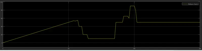
All these Drive cycles are connected with the help of Multi port switch which is used to switch between different drive cycles.

Driver control

In this model I have used PID controller as Driver control

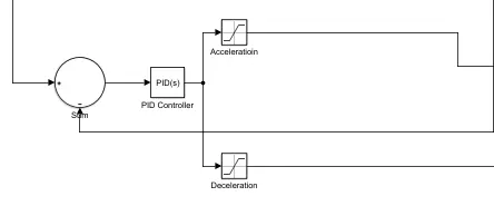
The Drive cycle input is given to sumation block from summation block it is given to PID controller. In order to set the acceleration and brake commands, I have used the saturation block. This block is used when we want to set limits for signals.

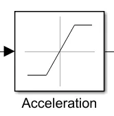
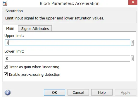
In the case of the accelerator command, I have set the limits between 0 and 1 by opening the saturation block parameters as shown below:

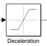
Another saturation block was used for the deceleration/brake commands which is shown below:

To create the deceleration commands, I have used a different set of limits between -1 and 0. This is shown in the image below

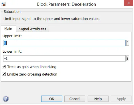
These limits ensure that there is no crossover with the acceleration commands.

Power Converter

Power converters are needed to provide power in the necessary magnitude and form from one component to another. In the system of an EV, power converters are used to supply the motor with the required power from the battery. In this model, I have used an H-Bridge block shown below:

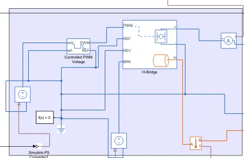
The H-Bridge block has 2 sides to it. The left side controls the voltage signals and the right side is for the terminals to provide the controlled voltage to the DC motor. The left side of the H-Bridge consists of ports which are explained below:

PWM - This stands for Pulse Width Modulation and provides voltage pulses to the H-Bridge in either the PWM mode or Average mode.

REF - This stands for reference.

REV - This stands for reverse.

BRK - This stands for brake.

Double-clicking the H-Bridge block, opens its block parameters shown in the image below:

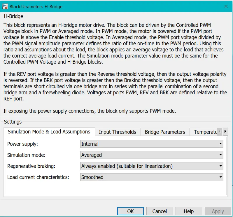
The main parameters are for the simulation mode and load assumptions of the H-Bridge. I have selected the H-Bridge to run on an "Internal" power supply with an "Averaged" simulation mode instead of the PWM mode. This is because using the PWM mode will result in significantly longer simulation times compared to using the averaged mode. I have enabled the regenerative braking mode and set the load current characteristics to the "Smoothed" option.

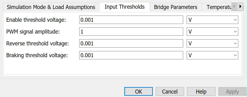
Input Thresholds

Bridge Parameters

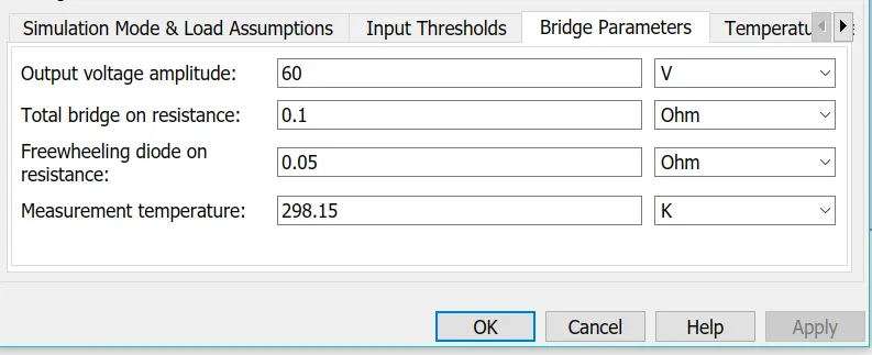
From the Bridge Parameters tab, we can modify parameters such as output voltage amplitude and total bridge on resistance.

Controlled PWM Voltage

Next, I have used a 'Controlled PWM Voltage' block to provide a controlled pulse width modulated voltage to the H-Bridge block. The block will output the PWM voltage through its 'PWM' and 'REF' ports which will feed in to the same ports found on the H-Bridge block. If the pulse is low the output voltage is considered 0V whereas if the pulse is high, the output voltage will be equal to the output voltage amplitude which was set to 60V in the H-Bridge block. The pulses of voltage created by this block are dependent on the duty cycle which is the ratio of the time that the switch is ON to the time taken for 1 cycle (which is the time for which the switch is ON and OFF). The duty cycle is set by the input of the controlled PWM voltage block.

The "Controlled PWM Voltage" block is shown below:

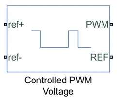
Double-clicking the block, opens the block parameters shown below:

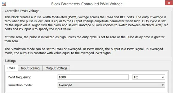
Under the "PWM" tab, I have chosen the 'Averaged' simulation mode so that the average value of the voltage pulses are generated and fed in to the H-Bridge. This will allow for quicker simulation times, just like for the H-Bridge block parameters.The remaining parameters of 'Input Scaling' and 'Output Voltage' are unchanged.

Controlled Voltage Source

The input ports of the controlled PWM voltage is connected to a controlled voltage source to provide the voltages to produce the voltage pulses to be fed in to the H-Bridge. For this, I have used the controlled voltage source block. This block is useful because it will provide the necessary voltage that is powerful enough to maintain the voltage at the output regardless of the current that passes through it.

The controlled voltage source block is shown below:

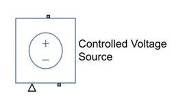
In this model, 2 controlled voltage sources have been used. One block is to provide the voltage for the acceleration of the vehicle and the other is to provide the voltage for the deceleration of the vehicle.

Electrical Reference

The electrical reference block is used to create a grounding effect for electrical circuits. Any model that uses electrical or electronics components will need to have atleast one electrical reference block in it. The electrical reference block is shown below:

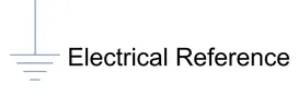
In this EV model, we are using this block to create an electrical ground between the controlled voltage source, controlled PWM voltage and the H-Bridge blocks.

Solver Configuration

The solver configuration block is used to solve any necessary equations in a model and in my case, I have used them in the connection to the 'REV' port of the H-Bridge block. The solver configuration block is shown below:

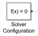
Battery System

The battery system is an essential part of the EV model as it will provide the electrical power required to power the DC motor. The components of the battery system are explained below:

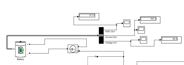
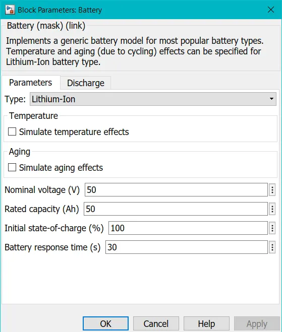
Here I have used Lithium ion battery

the parameters of the battery is shown below

SOC & Current

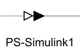
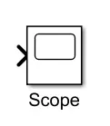
SOC stands for state of charge and it is a measurement of the available charge in a battery. When a battery is fully charged, it is considered to have a 100% charge and conversely 0% charge if fully discharged. In this EV model, I want to measure the current and the SOC of the battery as the simulation is run. For this, I have used a scope block which shows the output signal we wish to measure as a plot against time. 2 scopes have been used, one for the current and the other for the SOC. In order for this to be measured, we need to use a 'PS - Simulink converter' block. This is because the current signal is a physical one and we are measuring it as a logic signal in the SIMULINK workspace.

The PS-Simulink converter block is shown below:

The scope block is shown below:

Motor

For my EV model, I am using a DC motor block which is shown below:

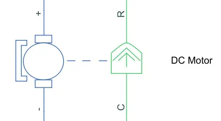
The left side of the motor represents the electrical part of the motor, whereas the right side represents the mechanical part. The mechanical part has 2 ports labelled C and R. C refers to the casing of the motor and R represents the rotation of the motor which produces the torque. The electrical part has 2 ends labelled with a positive and negative sign which represent the positive and negative terminals of the motor. Double-clicking the motor block opens the block parameters:

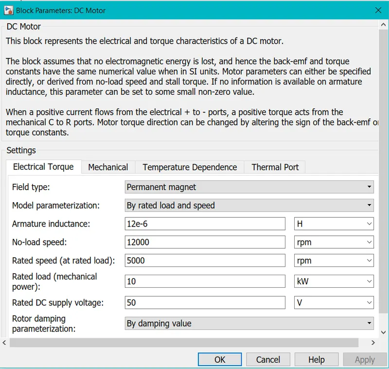
Under the "Electrical Torque" tab, we can model the electrical torque characteristics of the DC motor such as no-load speed, and rated DC supply voltage. I have used the values and settings shown in the image above.

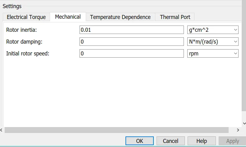
Under the "Mechanical" tab, we can model the mechanical torque characteristics such as rotor inertia and initial rotor speed. I have used the default values as shown in the image above.

In this model I have shown the thermal ports H which is used to measure the temperature of the Motor.

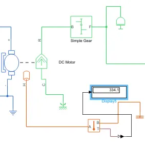
The H port is connected to temperature sensor to Display the temperature.

Vehicle Body

To model the body of the EV, we need to insert the vehicle body block shown in the image below:

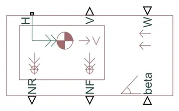
This block has 6 ports which represent various aspects of the modelling of the vehicle body:

• H - This stands for hub and allows us to connect the hubs of the wheels of the vehicle to the body.
• V - This stands for velocity and outputs the velocity of the vehicle.
• W - This represents wind velocity and allows us to model a headwind (against the front of the vehicle) acting on the velocity by giving a speed for it.
• NR - This represents the normal force on the rear wheels of the vehicle.
• NF - This represents the normal force on the front wheels of the vehicle.
• beta - This represents the grade (incline) of the surface that the vehicle travels on, as an angle to the horizontal.

Double-clicking the vehicle body block opens the block parameters shown below:

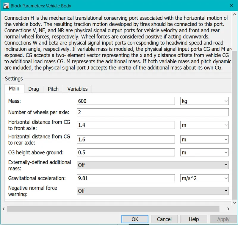
From the "Main" tab, here, we can model the basic parameters of the vehicle such as mass, number of wheels per axle and even gravitational acceleration. For my model, I am using a mass of 600kg, 2 wheels per axle (total of 3 wheels), and a gravitational acceleration of 9.81 metres per second squared.

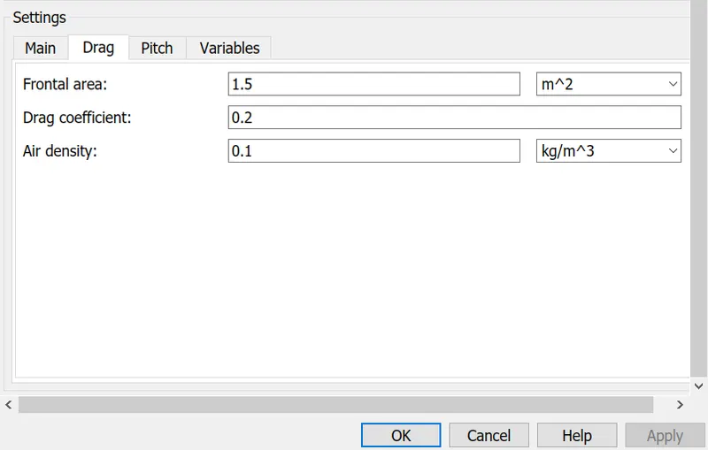
From the "Drag" tab, we can model the frontal area, drag coefficient, and the air density. I have used a frontal area, drag coefficient, and air density of 3, 0.3, and 1.18 respectively.

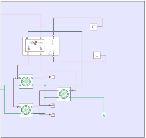
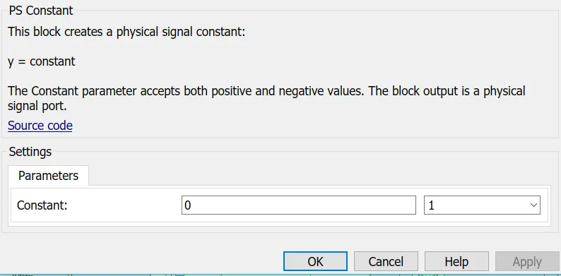
For wind velocity and Beta I Have given PS Constant.

Tires

In this model, I have used the "Magic Formula" tires. There are various tire blocks that can be used, but the advantage of the magic formula ones is that they enable us to model the longitudinal behavior of tires on a highway. This block is shown below:

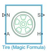
This block has 4 ports which represent various factors that can be modelled:

• N - This port represents the normal force on the tire and the downward direction is considered positive.
• S- This port represents the slip acting on the tire.
• A - This port represents the axle and is the mechanical rotational conserving port for the wheel axle.
• H - This port represents the hub and is the mechanical translational conserving port for the wheel hub.

Double-clicking the magic formula tire block, opens the block parameters window shown below:

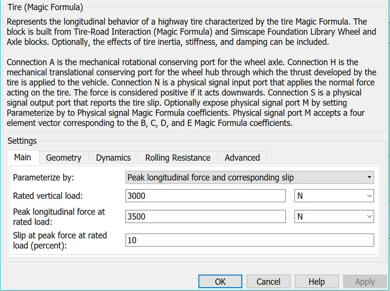
In the "Main" tab, we can model parameters such as tire nominal vertical load, and various coefficients. All values are kept as default

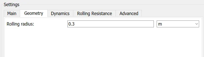
In the "Geometry" tab, we can model the rolling radius of the tire.

Gear

In this section, I have modelled the transmission of the EV. To simplify the transmission system of the EV model, I have used a "Simple Gear" block which uses a fixed gear ratio with no inertial effects. This block is shown below:

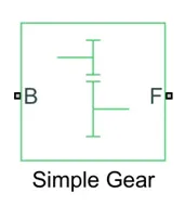
Double-clicking this block, opens the block parameters where we can model additional parameters of the gear.

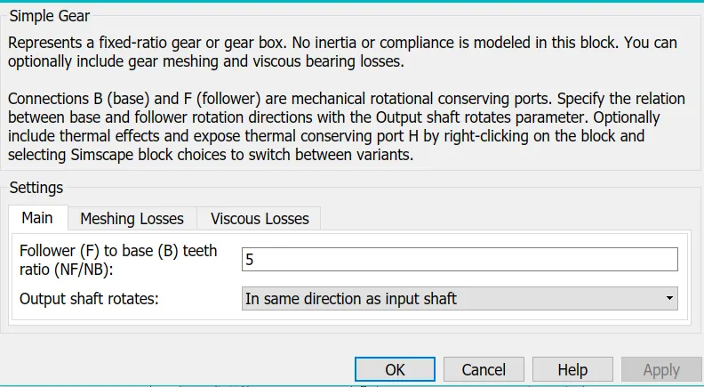
In the "Main" tab, we can model the follower to base teeth ratio and the direction of rotation of the output shaft

Speed Measurement

In order to measure the speed of the EV model, I needed to use the scope block once again. I modified the scope block to have 2 input ports where one port takes the output velocity signal from the vehicle body block and the other port takes the output signal from the drive cycle to the reference velocity port on the longitudinal driver block. This has been done so that the scope can show us the plots of the reference velocity and the actual velocity of the vehicle to see how they compare with each other.

Distance Measurement

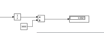
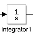
I have used the scope block and mathematical operator blocks to measure the distance travelled by the vehicle according to the drive cycle data. The area under a velocity time graph tells us the distance travelled by an object and so in my model. This means that the integral of the velocity with respect to time, gives us the distance travelled. So, I have implemented the integrator block to integrate the velocity signal that is output from the vehicle subsystem.

The integrator block is shown below:

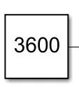
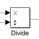
From the integrator block, I needed to use the 'Divide' block along with a 'Constant' block having a value of 3600 in order to convert the divide the integrated speed signal which is in kilometres per hour by 3600. This will give us the distance travelled in kilometres.

The constant block with a value of 3600:

The 'Divide' block:

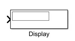
Finally, a 'Display' block is used to show the distance travelled as the simulation is running. The display block is shown below:

Result:

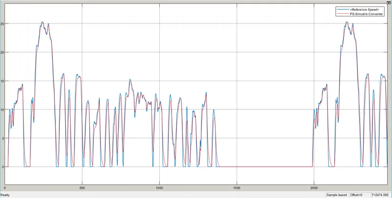
The blue line is graph of drive cycle source and red line shows the corresponding velocity graph. thus found that the drive cycle input and output velocity graph is almost overlapping on each other.

The variation of SOC & Battery current is shown below.

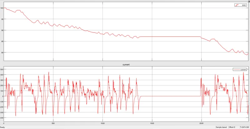
And the Distance travelled by the Vehicle is 17.76 km

CONCLUSION:

Thus all the objectives are achieved and the results are analysed properly.