Final Project: Electric Rickshaw modelling

Aim:

To create a detailed MATLAB model of an electric rickshaw (three wheel passenger vehicle).

Objectives:

To create an Electric rickshaw model with following details,

• Rear wheels driven by PM brushed type motor.
• Assume efficiency points of motor controller and motor.
• To create an excel sheet with all input and assumed data.
• Energy consumption values for three standard driving cycles.
• Temperature rise of motor and controller for 100Km constant driving at 45Kmph.

Introduction:

An electric autorickshaw is the combination of the following components and sub-systems

1. Drive cycle
2. Driver Controller
3. Battery
4. Power Controller
5. Motor and Gear system
6. Vehicle body

The block diagram of the electric rickshaw

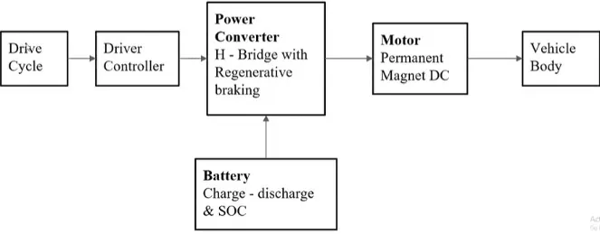
The current from the battery flows to DC Motor through the power converter to drive the motor. The required voltage will be controlled in the controller. The Controller will follow the given drive cycle reference and run the motor in the required rpm. Then the motor power is transmitted to the wheels of a vehicle through the gear box.

Matlab model

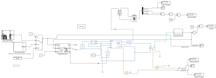
The vehicle get the type of drive cycle from the drive cycle source and it is given to the driver controller which controller the vehicle and also compares the refernce velocity and actual velocity. The H-bridge converter is connected to the PM brushed motor to produce the required voltage from the battery. The motor is connected to the gear box which further connected tires and vehicle body. The velocity from the vehicle body is given as feedback to the driver controller which compares the reference and actual velocity. Now let us look into each component and sub-system of the model.

Drive cycle:

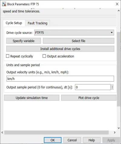
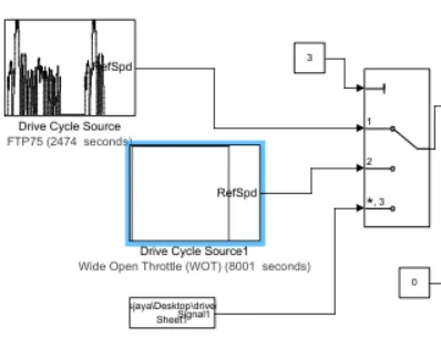
A driving cycle is a series of data points representing the speed of a vehicle versus time. It is assumed as driver input for the vehicle. Here we are considering 3 types of drive cycle out of which one is built-in FTP75 drive cycle with the help of ‘drive cycle source’ block and the other one was WOT type drive cycle with some pre-defined conditons and the third was an excel sheet consisting of velocity with time which was added with the help of ‘From Spreadsheet’ block.

1. FTP75drive cycle

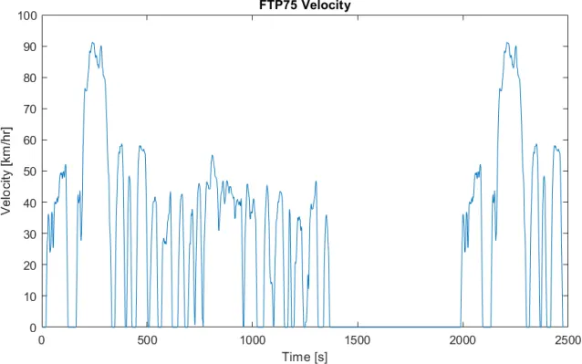
The Federal Test Procedure (FTP) is composed of the UDDS followed by the first 505 seconds of the UDDS. Though it was originally created as a reference point for fossil fuelled vehicles, the UDDS and thus the FTP-75, are also used to estimate the range in distance travelled by an electric vehicle in a single charge. The simulation time is 2474sec.

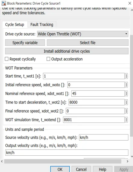
2. Wide Open Throttle(WOT)

As per given condition that the vehicle should run for 100km with the constant speed of 45kmph, then the time taken for the vehicle is

Time = distance/ speed

= = 8000 sec

So the simulation time is 8000sec.

User defined drive cycle

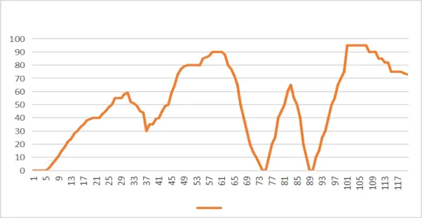
In this an excel is sheet is created which consists of velocity and time. The simulation time is 120sec. The excel sheet link is attached below.

https://in.docworkspace.com/d/sIO3T3PQto7jHiAY

The drivecycle is representes as

A multiport switch is used to select a drive cycle out of all the three drive cycle to simulate.

Driver Controller

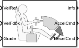
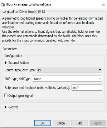
Drive cycle is connected to a longitudinal driver, it has six ports namely velocity reference, velocity feedback, grade, info, Acceleration, Deceleration.

VRef is given by the drive cycle data and VFdbk is given by the output of the vehicle body. These two will get compare and the acceleration or deceleration output will be given to the motor controller. Accelcmd is given the PWM generator block and deccelcmd is given to the regenerative port of the h-bridge which uses to generate regenerative braking. The grade is to give the input of gradeability to the driver block. The controll type used here is PI.

Power conroller system

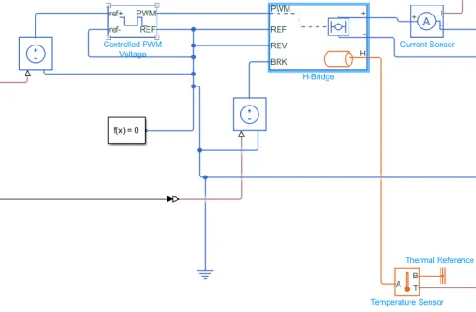
In this Controlled acceleration from driver subsystem is provided to controlled voltage source, the controlled voltage source converts the input of controlled acceleration signal to the equivalent voltage signal and output of controlled voltage source is provided to controlled PWM voltage block. Similarly, controlled braking signal is provided to another controlled voltage source and output of controlled voltage source is provided to H-bridge block.

• Controlled PWM Voltage

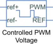
This block is used to create the pulse-width modulated (PWM) voltage. The block calculates the duty cycle based on the reference voltage across its ref+ and ref- ports.

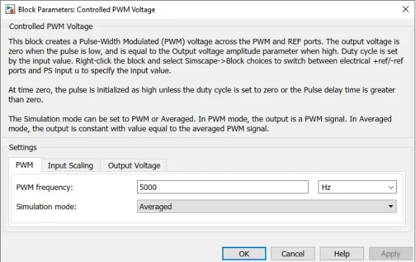
The Simulation mode is taken as Averaged.. In Averaged mode, the output is constant with value equal to the averaged PWM signal. The PWM frequency is taken as 5000 Hz.

• H- Bridge

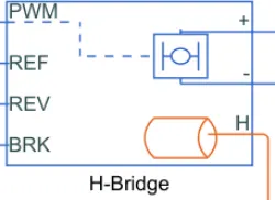
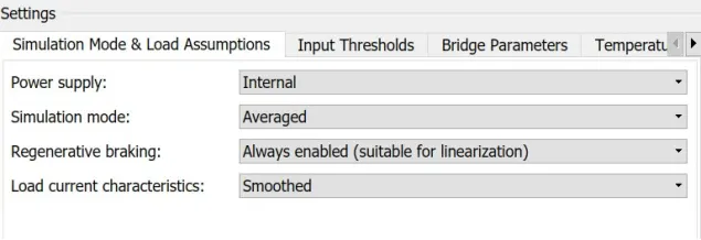
This block represents an H-bridge motor drive. The block can be driven by the Controlled PWM Voltage block in PWM or Averaged mode. In PWM mode, the motor is powered if the PWM port voltage is above the Enable threshold voltage. In Averaged mode, the PWM port voltage divided by the PWM signal amplitude parameter defines the ratio of the on-time to the PWM period. Using this ratio and assumptions about the load, the block applies an average voltage to the load that achieves the correct average load current. The Simulation mode parameter value must be the same for the Controlled PWM Voltage and H-Bridge blocks.

If the REV port voltage is greater than the Reverse threshold voltage, then the output voltage polarity is reversed. If the BRK port voltage is greater than the Braking threshold voltage, then the output terminals are short circuited via one bridge arm in series with the parallel combination of a second bridge arm and a freewheeling diode. Voltages at ports PWM, REV and BRK are defined relative to the REF port.

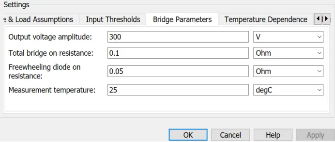
The voltage taken as 300v and temperature as 25degc.

• Current sensor

This is used to measure the current flowing through the H-bridge.

• Temperature sensor

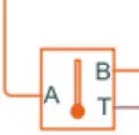
This block measures temperature in a thermal network. There is no heat flow through the sensor. The physical signal port T reports the temperature difference across the sensor. The measurement is positive when the temperature at port A is greater than the temperature at port B.

DC Motor:

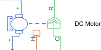
To convert the electrical energy to mechanical energy we use motors. In this electric vehicle model we have used PMDC brushed type motor. This motor can act as a generator also in case of regenerative braking. Also thermal port is added to this block by right-clicking on the model , and selecting simscape -> block choices -> show thermal port. This port will output the temperature of the motor.

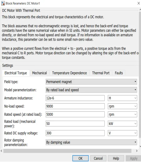
The rotor inertia taken is 0.01g*cm^2

And the initial temperature given is 25degC.

Battery system

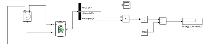
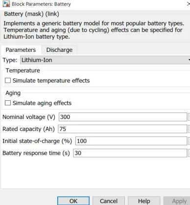
The battery is required to power the controller and motor. The controller uses the battery power according to produce the input given by the motor to obtain maximum speed. The battery is also used to power every electrical component in the vehicle. The battery has two stage one is charging and another one is discharging state. The battery is of 75Ah capacity.

The Nominal voltage of battery is 300 V, Initial SoC is of 100%.

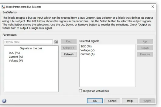
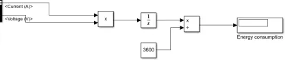
From this system we are going to observe the SOC and energy consumed. These are obtained by taking them through bus selector. Through bus selector SOC, current and voltage are obtained and from that Energy consumed is calculated.

Vehicle Body Subsystem

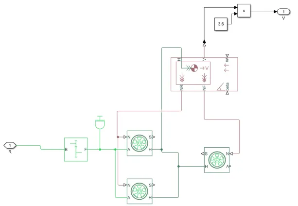
Here for this system motor will produce the rotational output which will give to the vehicle body and transmission system. The rotational output is taken by the gear system here to maintain the constant speed throughout the transmission without any loss in speed from the motor to tires. As mentioned the transmission created is a rear wheel drive where rear wheels axle is connected to the motor shaft.

• Gear Box

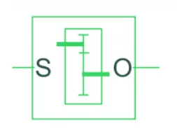
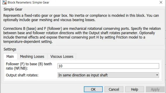
The gear box is characterized by its Gear ratio. The gear ratio is determined as the ratio of the input shaft angular velocity to that of the output shaft. Here Gear ratio is 10.

• Wheel

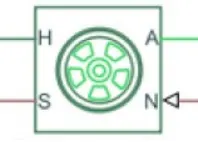
Tyre block Represents the longitudinal behaviour of a highway tire characterized by the tire Magic Formula. Connection A is the mechanical rotational conserving port for the wheel axle. Connection H is the mechanical translational conserving port for the wheel hub through which the thrust developed by the tire is applied to the vehicle. Connection N is a physical signal input port that applies the normal force acting on the tire. The force is considered positive if it acts downwards. Connection S is a physical signal output port that reports the tire slip. Optionally expose physical signal port M by right-clicking on the block and selecting Simscape block choices to switch between variants. Physical signal port M accepts a four-element vector corresponding to the B, C, D, and E Magic Formula coefficients.

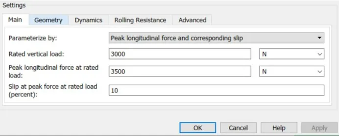
• Vehicle Body

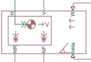
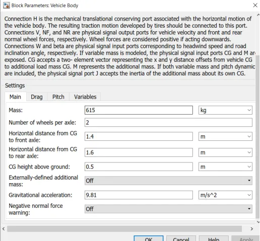
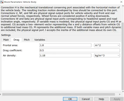
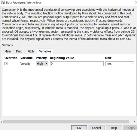
The vehicle body has an H-Hub, S- Tire slip, N- Normal force, A- axel connection, wind velocity, inclination angle. The tires hub is connected as a common node to the vehicle body. The vehicle body wind velocity is connected to a constant block and the beta-inclination angle is connected to another constant block where we can assign wind velocity and inclination angle as per requirement. Velocity is the output port where we can get at which speed the vehicle is moving. The velocity is taken out to the get the distance travelled and state of charge.

The vehicle parameters considered are

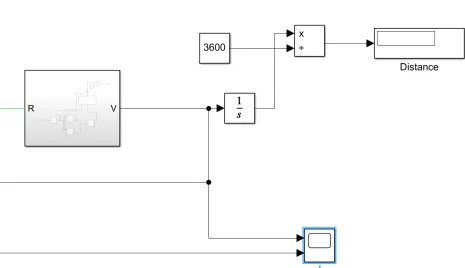
From the vehicle body, we get the velocity which is used to calculate the distance travelled by the vehicle with the help of the integrator and dividing it by 3600. And also the velocity is compared with reference velocity in the scope.

Results:

In this we are going to observe the comparison of ref velocity & actual velocity, SOC, temperature rise in motor and controller, energy consumed and distance travelled by the vehicle for each drive cycle.

For FTP75 Drive cycle

1. Reference vs Actual velocity

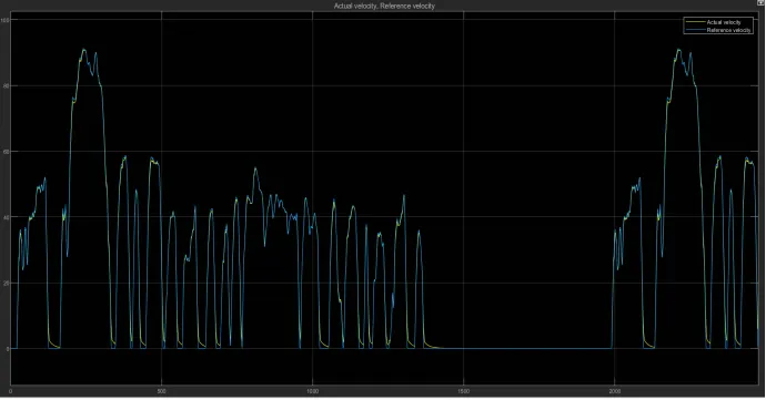
From the Reference and actual velocity graph we can observe that the electric rickshaw model that was designed had traced the FTP 75 drive cycle has almost accurately till the maximum speed it can achieve. The actual was quite than the reference at the time of deceleration to zero velocity.

2. SOC%

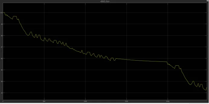
Now looking at the SOC graph we can see that almost 93.48% of the battery capacity is remaining after completing this drive cycle. And also we can see sudden spikes in that graph , these spikes represents the regenerative braking region. During which the SOC value increases.

3. Temperature of motor and controller

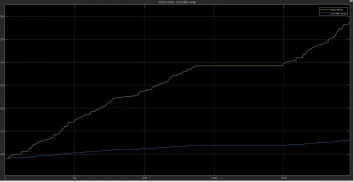
The rise in temperature of motor has reached almost 357 K which is initially at 298 K i.e., it is almost a temperature rise of about 58 K in motor. Temperature of motor rises when the vehicle is running and is constant when it stops.

And the rise in temperature of controller has reached almost 306 k which is initially at 299 k i.e., it is almost a temperature rise of about 7 K in motor which is very neglegible.

When compared to rise in temperature it is observed that there is more rise in temperature in motor. And from the graph for the two temperature values we can see that it is increasing as the distance covered increases , so if have to travel more distance than this drive cycle , then we should implement proper thermal system management.

4. Distance Travelled

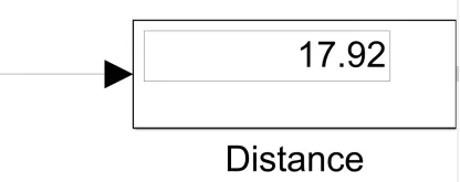
The distance travelled by the vehicle is 17.92 km

5. Energy consumed

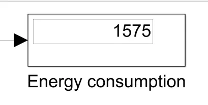
The energy consumed for completing the drive cycle is 1575Wh.

For Wide Open Throttle

1. Reference vs Actual velocity

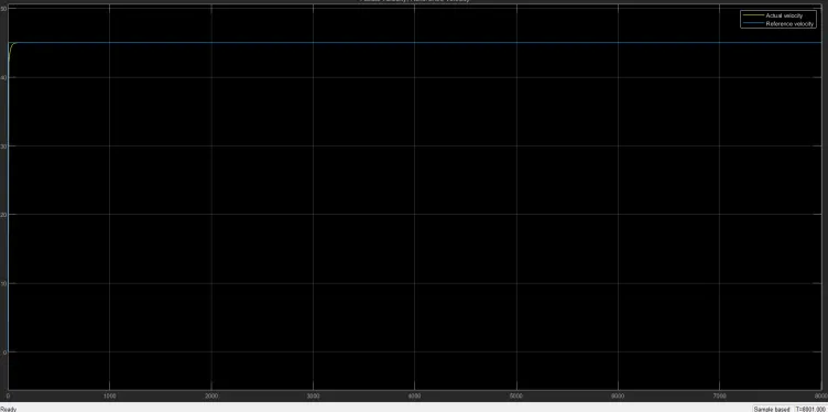
From the input vs output velocity graph for this drive cycle we can see that it follows the drive cycle and stays at 45 Kmph throughout the simulation time. At the beginning it took few seconds to reach 45 Kmph but after reaching it remained constant.

2. SOC%

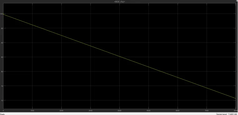
The SOC graph for this drive cycle is pretty straight forward because there is no braking or deceleration taking place . So the SOC value decreased proportional to the distance covered. The remaining SOC is almost 70%.

3. Temperature of motor and controller

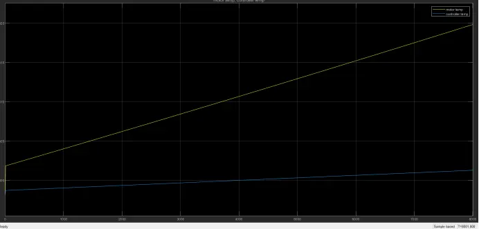
The Temperature rise in motor and controller temperature has reached 319 K and 301 K respectively which is initially 298 K.

4. Distance Travelled

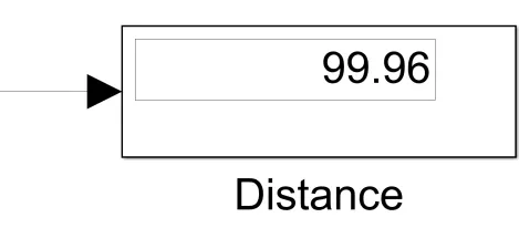
The distance travelled by the vehicle after completeing the drive cycle is almost equal to 100km

5. Energy consumed

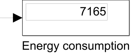
The energy consumed by the vehicle for completing the drive cycle is 7165Wh.

For User defined drive cycle

1. Reference vs Actual Velocity

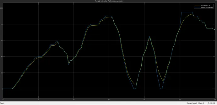
From the plot we can observe that the actual velocity has almost traced the reference velocity but not accurately. Here the actual velocity response is slow at the sharp acceleration and deceleration when compared to the reference.

2. SOC%

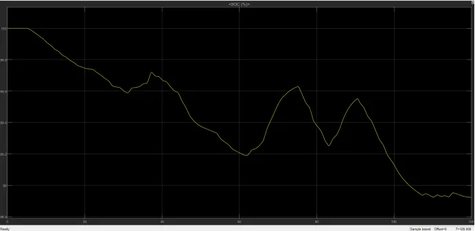
The SOC graph didn’t had much change and the battery percentage remaining was 98%. But from this SOC graph we can clearly see the point at which regenerative braking takes place , these are the points where the graph increases.

3. Temperature of motor and controller

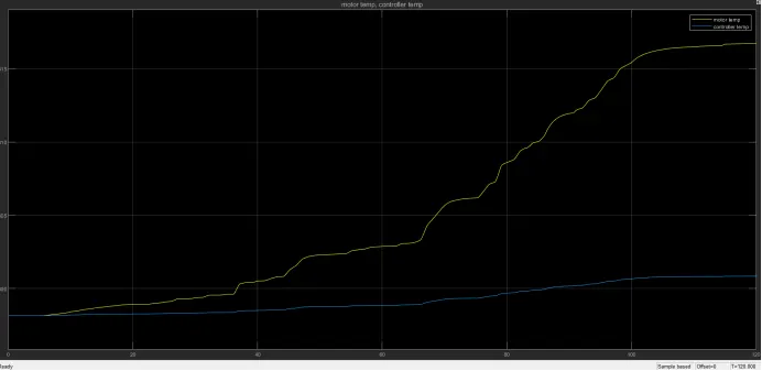
And the motor and controller temperature reached 316 K and 300 K respectively which is initially 298 K. These are very low values , and this is because the vehicle hasn’t travelled for long distance.

4. Distance travelled

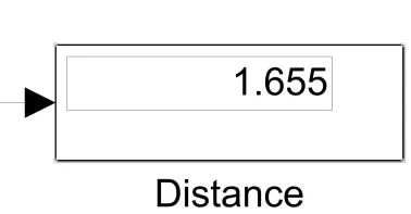
The drive cycle is very small and it covers only a distance of 1.655Km

5. Energy consumed

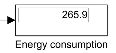
The energy consumed for completing the drive cycle is 265.9Wh.

Conclusion:

Hence, Created a MATLAB model of an Electric Rickshaw (three wheel passenger vehicle) by using PM Brushed DC Motor.

Detremined the variations of Temperature of Motor and controller, SoC% and Energy consumed, distance travelled by the by vehicle for all the three Reference Drive cycles i.e.; FTP75, WOT, User defined.