Final Project: Electric Rickshaw modelling
Aim: Design of an Electric Rickshaw using MATLAB Simulink.
Abstract
- We are going to simulink a MATLAB model of the Electric Rikshaw by using a PM brushed type DC motor
- And a suitable Lithium-Ion battery for the Rikshaw. We will know about what is Electric Rikshaw and how it works, the benefits of Electric Rikshaw.
- Then we are going to build a model of simulink for an actual EV Rickshaw with suitable blocks from the powertrain block set.
- Our main purpose is to check performance of our built model of an Ev Rikshaw .
- And how our simulink model performs for any three different standard driving cycles showing energy consumption
- The temperature rise of motor and controller for vehicle cover around 100 km at constant speed driving 45 kmph.
Objectives :
Create a detailed MATLAB model of an electric rickshaw (three wheel passenger vehicle) as per details below :
- Rear wheels driven by PM brushed type motor
- Assume efficiency points of motor controller and motor
- Make an excel sheet of all input and assumed data
- Results: For any three standard driving cycles show energy consumption, temperature rise of motor and controller for 100 km constant speed driving at 45 kmph.
Methodology :
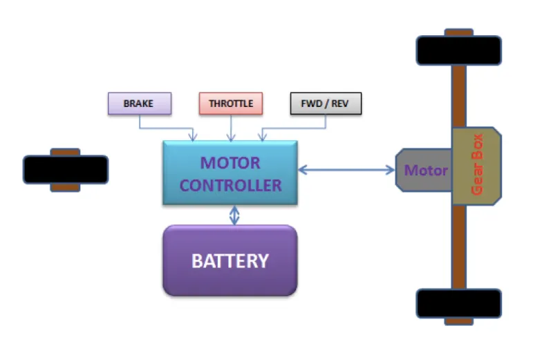
- The electric vehicle Rikshaw consists of a battery, motors, and controller then it generates propulsion power.
- To design any vehicle 1st we have to calculate propulsion power, then the motor is selected.
- Lastly based on the motor rating or operating range and no km/charge we want to depend on everything battery capacity and then battery capacity is selected. So the Design flow of vehicle engineer has to be like the following :
- Identify what amount of propulsion power required.
- What is the best suitable motor for that propulsion power.
- Then type of battery and range of battery according to the range.
Introduction :
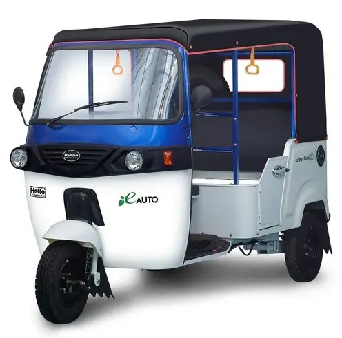
- E rickshaws are now fairly popular amongst Indian rickshaw drivers and have created new opportunities for people, as they require a minimum investment to earn a living.
- They offer huge returns in less time and are easy to operate and has low maintenance and running cost.
- A lot of variants are available these days, most of them started as low-quality products and were imported from China.
- These days Indian e rickshaws have been developed offering a higher quality and better services at an equivalent cost.
- E rickshaws can provide a decent income since the battery charging cost is far lower than any other fuel, new material such as fiberglass has been introduced in them since the material provides high strength, durability and lighter than metals.
- E Rickshaw in India are built over tubular chassis, a body is kept a light in weight in order to increase the life of the battery, the main electronic components that make the drive are motor, controller, harness, batteries and the throttle.
- The mismatch between any of these components is undesirable and may reduce performance.
Block diagram of E Rikshaw
Manufacturing
- The chassis is the main part which ensures drive quality and safety of the vehicle, is made of mild steel, a low-quality chassis should never be used, the chassis is often built without proper knowledge, causing an imbalance in the drive, and often causing the vehicle to pivot very easily, the chassis manufactured by professional E Rickshaw Manufacturer are better as quality measures are often ignored by others, and are often built without welding fixtures of any kind.
- The chassis inaccurately made, will have handling problems, will be damaged easily, and corrosion may occur if not treated for resisting certain chemicals(from the battery or otherwise) or moisture.
- The low weight of a body is desirable, which can be done by good designing, ensuring quality check, using a material such as F.R.P, aluminum, composite materials, and low-density metals.
- A very good alternative is F.R.P which is strong, non conducting, cheap, lightweight, highly durable, resistant to fire, withstands weather and is easily repaired in case of damage.
- The body is attached to chassis by the means of bolts, in some cases welded, which is not recommended. The body should be built to keep in mind quality and design which is aerodynamic and ensures driver safety.
- Better quality bodies last for years whereas low-quality body will last no longer than 10 to 15 months. In this case, F.R.P is extremely desirable since the life of the body is 10s of years.
- Electrical parts are recommended to be tight, use high-quality couplers to ensure proper connection and insulate connection to prevent water and moisture.
- Electrical components used of higher quality will lower resistance and heat losses and increase efficiency.
- The motor power used in most e rickshaws is 650W to 1250W, the latest government norms allow it to be 650W, most of them run on 850W and higher, which adversely affects the battery life.
- The controller used is ~ 40A, 48V output, uses 14, 18 or 24 MOSFETs and powers all electric components.
- A good quality controller must be used to increase the performance of the motor and other overheating issues.
- A controller should be installed with electrical brake cut off, and which are removed by common rickshaw mechanics in order to achieve a continuous torque or improper functioning of the brakes.
- The braking system is mechanical drum brakes. Service and maintenance are required for proper vehicle functioning, the improper brake adjustments may heat up the motor and controllers and damage brake shoes, it may also reduce the mileage of the vehicle.
- The batteries used in e rickshaws are lead acid, they provide low-cost alternative, they range from 80A to 120A nowadays, a larger battery with more capacity is used, but adversely it can increase weight and reduce mileage, to prevent it the ratio of weight and AH(measure of battery capacity) must be maintained, we recommend to use not more than 110AH batteries as they exceed 125kg, deep discharge batteries made for electric vehicles may be used depending on the customer’s preference.
- To main life, a low amperage charger ~10 to 15A should be used, a charger with current and voltage maintained is preferred to prevent bulging and higher cycles.
- Every aspect of an electric vehicle, if engineered, designed and manufactured with quality will improve battery life, vehicle life and contribute to a higher profit over time.
- Electric E-Rickshaw is also known as electric tuk-tuk, e-rickshaw and auto which are going more popular after 2018 in Indian market. This E-rickshaw is best alternative of petrol/ CNG auto rickshaw and human or horse pulled rickshaws because of their low fuel cost, zero emissions and less human efforts.
- The electrical system used in Indian version is 48VDC can run 90– 100 km/full charge, top speed 25 km/hour and this electric motor power ranging from 650-1400 Watts; the battery takes 8–10 hrs to become fully charged. Basic seating capacity is driver plus 4 passenger total 5 persons.
- Here basically, e-rickshaw is designed in CREO and MATLAB Simulink. In the designed electric rickshaw main blocks are battery, drive cycle, controlled, DC Motor, Vehicle body and transmission system. Drive cycle is the input of human effort that how he is going to drive his actual cycle. We can use drive cycle like FTP75, WOT or by using Excel.
- The main objective of this project is to obtain speed by driver, to estimate the temperature of motor and controller, to estimate the state of charge (SOC) and distance travel by the vehicle. There is a SOC block that will estimate the state of charge of battery, distance is calculated by speed and time parameter for all the three Drive cycle.
Specifications Of Electric Rikshaw and their components
Battery
Battery type : Lithium Ion
Nominal voltage (V) : 48.
Rated capacity (Ah) : 100.
Initial state-of-charge (%) : 100
Battery response time (s):10.
Motor
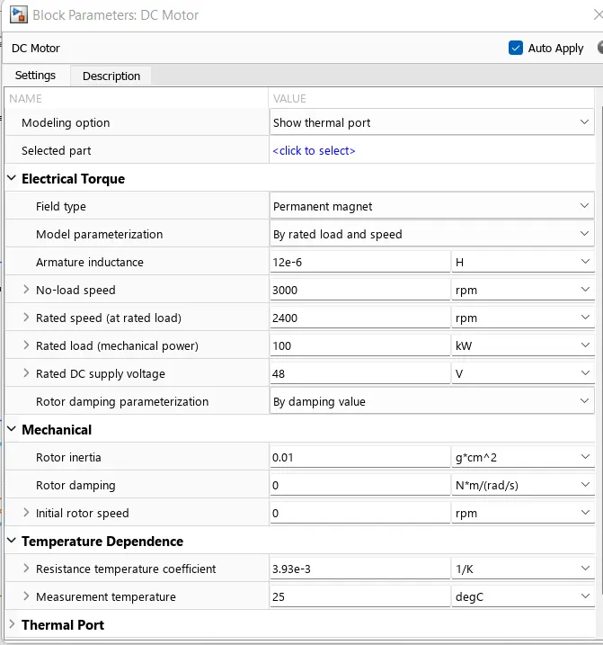
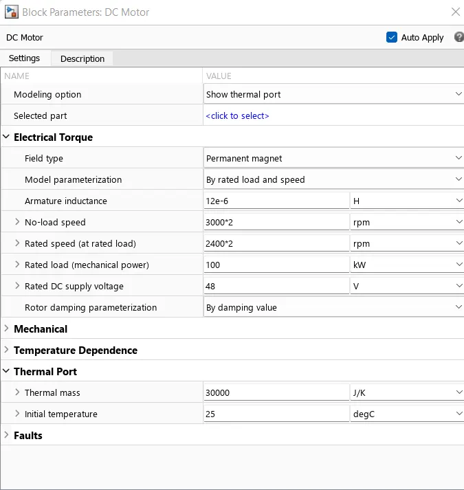
Field type : Permanent magnet
Model Parameterization : By rated load and speed.
Armature inductance : 12e-6 H.
No-load speed : 3000 rpm.
Rated load (mechanical power) : 100 kw.
Rated DC supply voltage : 48V.
Vehicle body
Mass : 500.
Number of wheels per axle : 2.
Horozontal distance from CG to front axle : 1.4.
Horozontal distance from CG to rear axle : 1.6.
Gravitational acceleration : 9.81.
Simulink model of an E Rikshaw
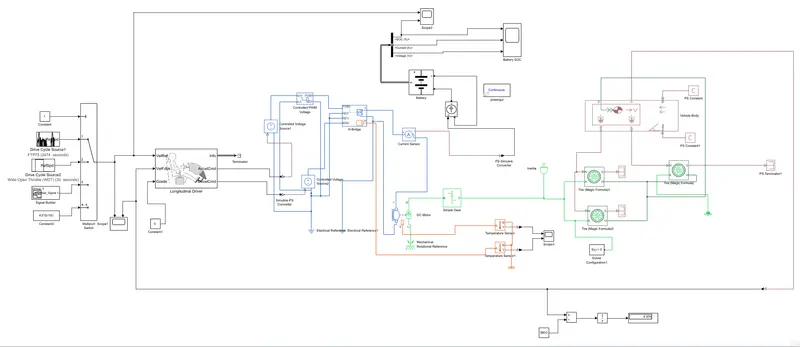
Blocks used for simulink model of an E Rickshaw with their functions.
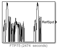
- Drive cycle cource
Description
The Drive Cycle Source block generates a standard or user-specified longitudinal drive cycle. The block output is the specified vehicle longitudinal speed, which you can use to:
-
Predict the engine torque and fuel consumption that a vehicle requires to achieve desired speed and acceleration for a given gear shift reference.
-
Produce realistic velocity and shift references for closed loop acceleration and braking commands for vehicle control and plant models.
-
Study, tune, and optimize vehicle control, system performance, and system robustness over multiple drive cycles.
Identify the faults within tolerances specified by standardized tests, including:
- EPA dynamometer driving schedules1
- Worldwide Harmonised Light Vehicle Test Procedure (WLTP) laboratory tests2
For the drive cycles, you can use:
-
Drive cycles from predefined sources. By default, the block includes the
FTP–75drive cycle. To install additional drive cycles from a support package, see Install Drive Cycle Data. The support package has drive cycles that include the gear shift schedules, for exampleJC08andCUEDC. -
Workspace variables that define your own drive cycles.
-
.
mat, .xls, .xlsx, or .txtfiles. -
Wide open throttle (WOT) parameters, including initial and nominal reference speed, deceleration start time, and final reference speed.
To achieve the goals listed in the table, use the specified Drive Cycle Source block parameter options.
- Signal builder

The Signal Builder block allows you to create interchangeable groups of signal sources and quickly switch the groups into and out of a model. Signal groups can greatly facilitate testing a model, especially when used in conjunction with Simulink assertion blocks and the optional Model Coverage Tool.
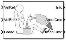
- Longitudinal driver
-
Vehicle Dynamics Blockset / Vehicle Scenarios / Driver
Description
The Longitudinal Driver block implements a longitudinal speed-tracking controller. Based on reference and feedback velocities, the block generates normalized acceleration and braking commands that can vary from 0 through 1. You can use the block to model the dynamic response of a driver or to generate the commands necessary to track a longitudinal drive cycle.
Configurations
Use the External Actions parameters to create input ports for signals that can disable, hold, or override the closed-loop acceleration or deceleration commands. The block uses this priority order for the input commands: disable (highest), hold, override.
- Controlled voltage source

Description
The Controlled Voltage Source block converts a Simulink input signal into an equivalent voltage source. The generated voltage is driven by the input signal of the block.
You can initialize the Controlled Voltage Source block with a specific AC or DC voltage. If you want to start the simulation in steady state, the Simulink input must be connected to a signal that begins the simulation as a sinusoidal or DC waveform that corresponds to the initial values.
- Controlled PWM voltage
-
Simscape / Electrical / Integrated Circuits

Description
The Controlled PWM Voltage block represents a pulse-width modulated (PWM) voltage source. You can model electrical or physical signal input ports by setting the Modeling option parameter to either:
-
Electrical input ports— The block calculates the duty cycle based on the reference voltage across its ref+ and ref- ports. This option is the default. -
PS input— Specify the duty cycle value directly by using an input physical signal port.
If you set Modeling option to Electrical input ports, the demanded duty cycle is
100∗(Vref−Vmin)/(Vmax−Vmin)* percent
where:
-
Vref is the reference voltage across the ref+ and ref- ports.
-
Vmin is the minimum reference voltage.
-
Vmax is the maximum reference voltage.
The value of the Output voltage amplitude parameter determines amplitude of the output voltage.
At time zero, the pulse is initialized as high, unless the Pulse delay time parameter is greater than zero, or the demanded duty cycle is zero.
You can use parameters Pulse delay time and Pulse width offset to add a small turn-on delay and a small turn-off advance. This can be useful when fine-tuning switching times so as to minimize switching losses.
In PWM mode, the block has two options for the type of switching event when moving between output high and output low states:
-
Asynchronous – Best for variable-step solvers— Asynchronous events are better suited to variable step solvers, because they require fewer simulation steps for the same level of accuracy. In asynchronous mode the PWM switching events generate zero crossings, and therefore switching times are always determined accurately, regardless of the simulation maximum step size. -
Discrete—time – Best for fixed-step solvers— Discrete-time events are better suited to fixed-step operation, because then the switching events are always synchronized with the simulation step. Using an asynchronous implementation with fixed-step solvers may sometimes result in events being up to one simulation step late. For more information, see Simulating with Fixed Time Step — Local and Global Fixed-Step Solvers.
If you use a fixed-step or local solver and the discrete-time switching event type, the following restrictions apply to the Sample time parameter value:
-
The sample time must be a multiple of the simulation step size.
-
The sample time must be small compared to the PWM period, to ensure sufficient resolution.
- Current sensor
Simscape / Electrical / Sensors & Transducers

Description
The Current Sensor block represents an ideal current sensor, that is, a device that converts current measured in any electrical branch into a physical signal proportional to the current.
Use the + and - ports to connect the sensor in series with the other blocks in the branch where you want to measure the current. Port I outputs the measurement result as a physical signal. Use a PS-Simulink Converter block to connect this port to Simulink blocks, such as Scope or Display.
- Controlled current source

Description
The Controlled Current Source block converts the Simulink® input signal into an equivalent current source. The generated current is driven by the input signal of the block. The positive current direction is as shown by the arrow in the block icon.
You can initialize the Controlled Current Source block with a specific AC or DC current. If you want to start the simulation in steady state, the block input must be connected to a signal starting as a sinusoidal or DC waveform corresponding to the initial values.
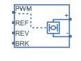
- H-Bridge
Description
The H-Bridge block represents an H-bridge motor driver. The block has the following two Simulation mode options:
-
PWM— The H-Bridge block output is a controlled voltage that depends on the input signal at the PWM port. If the input signal has a value greater than the Enable threshold voltage parameter value, the H-Bridge block output is on and has a value equal to the value of the Output voltage amplitude parameter. If it has a value less than the Enable threshold voltage parameter value, the block maintains the load circuit using one of the following three Freewheeling mode options:-
Via one semiconductor switch and one freewheeling diode -
Via two freewheeling diodes -
Via two semiconductor switches and one freewheeling diode
-
- Battery

A battery is a source of electric power consisting of one or more electrochemical cells with external connections for powering electrical devices.
- Powergui

Description
The powergui block allows you to choose one of these methods to solve your circuit:
-
Continuous, which uses a variable-step solver from Simulink.
-
Discretization of the electrical system for a solution at fixed time steps
-
Continuous or discrete phasor solution
The powergui block also opens tools for steady-state and simulation results analysis and for advanced parameter design.
You need the powergui block to simulate any Simulink model containing Simscape™ Electrical™ Specialized Power Systems blocks. It stores the equivalent Simulink circuit that represents the state-space equations of the model.
When using one powergui block in a model:
-
Place the powergui block in the top-level diagram for optimal performance.
-
Make sure that the block is named
powergui.
- Scope

scopes provide several methods for displaying simulation data and capturing the data for later analysis
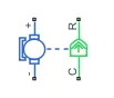
- DC motor
- Library:
-
Simscape / Electrical / Electromechanical / Brushed Motors
Description
The DC Motor block represents the electrical and torque characteristics of a DC motor using the following equivalent circuit model:
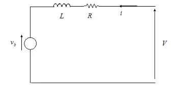
You specify the equivalent circuit parameters for this model when you set the Model parameterization parameter to By equivalent circuit parameters. The resistor R corresponds to the resistance you specify in the Armature resistance parameter. The inductor L corresponds to the inductance you specify in the Armature inductance parameter.
You can specify how to generate the magnetic field of the DC motor by setting the Field type parameter to the desired option. The permanent magnets in the motor induce the following back emf vb in the armature:
vb=kvω
where kv is the Back-emf constant and ω is the angular velocity. The motor produces the following torque, which is proportional to the motor current i:
TE=kti
where kt is the Torque constant. The DC Motor block assumes that there are no electromagnetic losses. This means that mechanical power is equal to the electrical power dissipated by the back emf in the armature
- Simple gear

Description
The Simple Gear block represents a gearbox that constrains the connected driveline axes of the base gear, B, and the follower gear, F, to corotate with a fixed ratio that you specify. You choose whether the follower axis rotates in the same or opposite direction as the base axis. If they rotate in the same direction, the angular velocity of the follower, ωF, and the angular velocity of the base, ωB, have the same sign. If they rotate in opposite directions, ωF and ωB have opposite signs. You can easily add and remove backlash, faults, and thermal effects
- Inertia
-
Simscape / Foundation Library / Mechanical / Rotational Elements

Description
The Inertia block represents an ideal mechanical translational inertia that is described with the following equation:
T=J (dω/dt)
where:
-
T is inertia torque.
-
J is inertia.
-
ω is angular velocity.
-
t is time.
By default, the block has one mechanical translational conserving port. The block positive direction is from its port to the reference point. This means that the inertia torque is positive if inertia is accelerated in the positive direction.
In some applications, it is customary to display inertia in series with other elements in the block diagram layout. To support this use case, the Number of graphical ports parameter lets you display a second port on the opposite side of the block icon. The two-port variant is purely graphical: the two ports have the same angular velocity, so the block functions exactly the same whether it has one or two ports. The block icon changes depending on the value of the Number of graphical ports parameter.
- Vehicle body
Simscape / Driveline / Tires & Vehicles
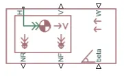
Description
The Vehicle Body block represents a two-axle vehicle body in longitudinal motion. The vehicle can have the same or a different number of wheels on each axle. For example, two wheels on the front axle and one wheel on the rear axle. The vehicle wheels are assumed identical in size. The vehicle can also have a center of gravity (CG) that is at or below the plane of travel.
The block accounts for body mass, aerodynamic drag, road incline, and weight distribution between axles due to acceleration and road profile. Optionally include pitch and suspension dynamics. The vehicle does not move vertically relative to the ground.
The block has an option to include an externally-defined mass and an externally-defined inertia. The mass, inertia, and center of gravity of the vehicle body can vary over the course of simulation in response to system changes.
Model
The vehicle axles are parallel and form a plane. The longitudinal, x, direction lies in this plane and perpendicular to the axles. If the vehicle is traveling on an incline slope, β, the normal, z, direction is not parallel to gravity but is always perpendicular to the axle-longitudinal plane.
- Simulink PS converter

Description
The Simulink-PS Converter block converts the input Simulink signal into a physical signal. Use this block to connect Simulink sources or other Simulink blocks to the inputs of a Simscape physical network.
- PS simulink converter

Description
The PS-Simulink Converter block converts a physical signal into a Simulink output signal. Use this block to connect outputs of a Simscape physical network to Simulink scopes or other Simulink blocks.
- Terminator

Description
Use the Terminator block to cap blocks whose output ports do not connect to other blocks. If you run a simulation with blocks having unconnected output ports, Simulink® issues warning messages. Using Terminator blocks to cap those blocks helps prevent warning messages.
- PS terminator

Description
Use the PS Terminator block to cap physical signal output ports that do not connect to other blocks.
Unlike conserving ports in physical modeling, or Simulink® output ports, unconnected physical signal output ports do not generate warnings. However, you can use a PS Terminator block for clarity, to indicate that the signal was not inadvertently left unconnected.
- PS constant

Description
The PS Constant block generates a physical signal of a constant value. You specify the value and unit of the signal as the Constant parameter.
- Temperature sensor
Thermal Sensors

Description
The Temperature Sensor block represents an ideal temperature sensor, that is, a device that determines the temperature differential measured between two points without drawing any heat.
Connections A and B are thermal conserving ports that connect to the two points where temperature is being monitored. Port T is a physical signal port that outputs the temperature differential value.
The block positive direction is from port A to port B. The measured temperature is determined as T = TA – TB.
- Thermal reference

Description
The Thermal Reference block represents a thermal reference point, that is, a point with an absolute zero temperature, with respect to which all the temperatures in the system are determined.
- Electrical reference

Description
The Electrical Reference block represents an electrical ground. Electrical conserving ports of all the blocks that are directly connected to ground must be connected to an Electrical Reference block. A model with electrical elements must contain at least one Electrical Reference block.
- Mechanical rotational reference

Description
The Mechanical Rotational Reference block represents a reference point, or frame, for all mechanical rotational ports. All rotational ports that are rigidly clamped to the frame (ground) must be connected to a Mechanical Rotational Reference block.
- Solver configuration

Description
Each physical network represented by a connected Simscape™ block diagram requires solver settings information for simulation. The Solver Configuration block specifies the solver parameters that your model needs before you can begin simulation.
Each topologically distinct Simscape block diagram requires exactly one Solver Configuration block to be connected to it.
- Integrator

Description
The Integrator block outputs the value of the integral of its input signal with respect to time.
Simulink treats the Integrator block as a dynamic system with one state. The block dynamics are given by:
{˙x(t)=u(t)
y(t)=x(t) x(t0)=x0
where:
-
u is the block input.
-
y is the block output.
-
x is the block state.
-
x0 is the initial condition of x.
While these equations define an exact relationship in continuous time, Simulink uses numerical approximation methods to evaluate them with finite precision. Simulink can use several different numerical integration methods to compute the output of the block, each with advantages in particular applications. Use the Solver pane of the Configuration Parameters dialog box (see Solver Pane) to select the technique best suited to your application.
The selected solver computes the output of the Integrator block at the current time step, using the current input value and the value of the state at the previous time step. To support this computational model, the Integrator block saves its output at the current time step for use by the solver to compute its output at the next time step. The block also provides the solver with an initial condition for use in computing the block's initial state at the beginning of a simulation. The default value of the initial condition is 0. Use the block parameter dialog box to specify another value for the initial condition or create an initial value input port on the block.
Use the parameter dialog box to:
-
Define upper and lower limits on the integral
-
Create an input that resets the block's output (state) to its initial value, depending on how the input changes
-
Create an optional state output so that the value of the block's output can trigger a block reset
Use the Discrete-Time Integrator block to create a purely discrete system.
- Divide

Description
The Divide block outputs the result of dividing its first input by its second. The inputs can be scalars, a scalar and a nonscalar, or two nonscalars that have the same dimensions. This block supports only complex input values at division ports when all ports have the same single or double data type.
The Divide block is functionally a Product block that has two block parameter values preset:
-
Multiplication —
Element-wise(.*) -
Number of Inputs —
*/
Setting nondefault values for either of those parameters can change a Divide block to be functionally equivalent to a Product block or a Product of Elements block.
- Display
Description
The Display block shows the value of the input data. You can specify the frequency of the display. For numeric input data, you can also specify the format of display.
If the block input is an array, you can resize the block vertically or horizontally to show more than just the first element. If the block input is a vector, the block sequentially adds display fields from left to right and top to bottom. The block displays as many values as possible. A black triangle indicates that the block is not displaying all input array elements.
The Display block shows the first 200 elements of a vector signal and the first 20 rows and 10 columns of a matrix signal.
- Tire

Description
The Tire (Magic Formula) block represents a tire with longitudinal behavior given by the Magic Formula [1], an empirical equation based on four fitting coefficients. The block can model tire dynamics under constant or variable pavement conditions.
The longitudinal direction of the tire is the same as its direction of motion as it rolls on pavement. This block is a structural component based on the Tire-Road Interaction (Magic Formula) block.
To increase the fidelity of the tire model, you can specify properties such as tire compliance, inertia, and rolling resistance. However, these properties increase the complexity of the tire model and can slow down simulation. Consider ignoring tire compliance and inertia if simulating the model in real time or if preparing the model for hardware-in-the-loop (HIL) simulation.
Tire Model
The Tire (Magic Formula) block models the tire as a rigid wheel-tire combination in contact with the road and subject to slip. When torque is applied to the wheel axle, the tire pushes on the ground (while subject to contact friction) and transfers the resulting reaction as a force back on the wheel. This action pushes the wheel forward or backward. If you include the optional tire compliance, the tire also flexibly deforms under load.
Subsystems of simulink model of an E Rikshaw
Simulink model of an E Rickshaw with subsystems.
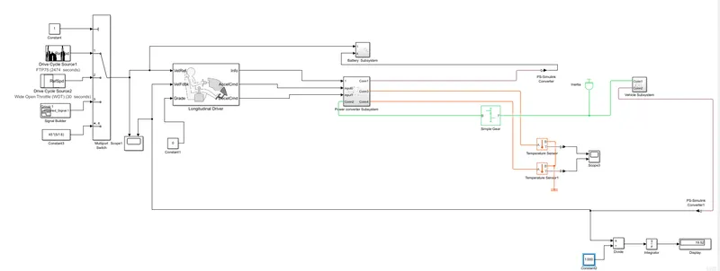
Subsystem of Vehicle body of an E Rikshaw
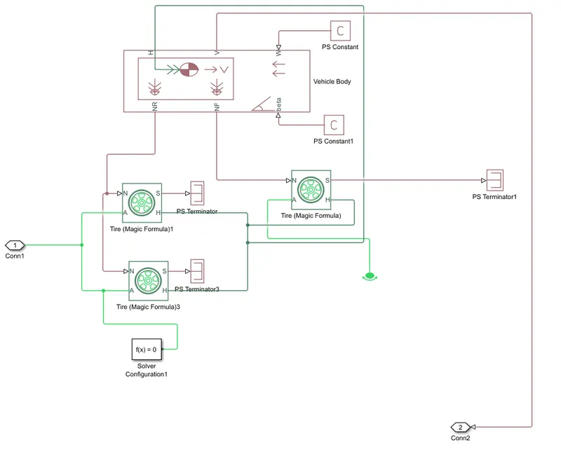
Explanation
- Motor will produce the rotational output which will give to the vehicle body and transmission system. The rotational output is taken by the gear system here to maintain the constant speed throughout the transmission without any loss in speed from the motor to tires.
- Below is a diagram that is how it is how it inside the vehicle body and transmission system and in the main design, it is referred just only as a transmission system.
- Here I created a Rear wheel drive transmission system.
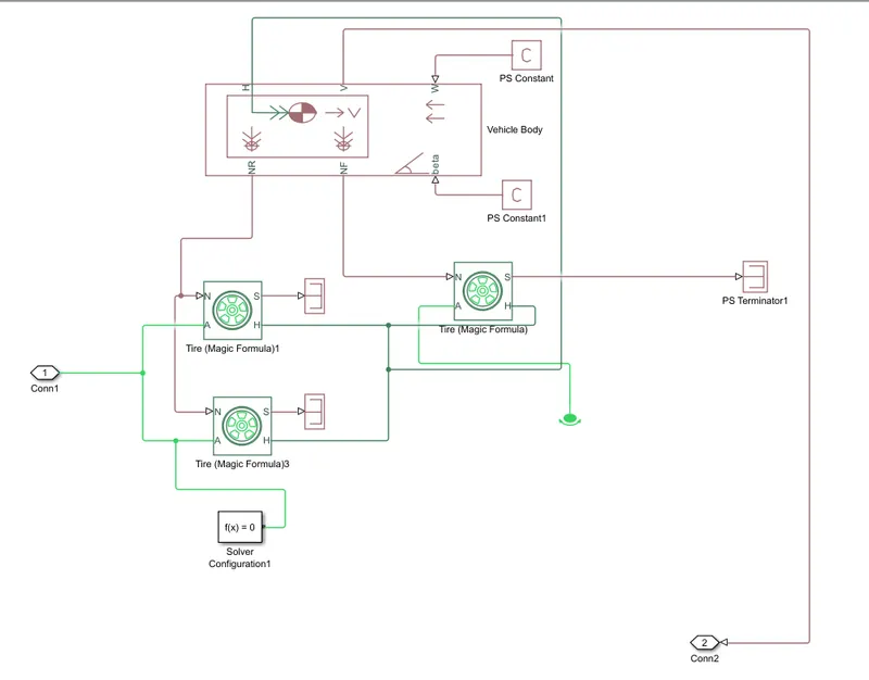
- The gear output is given to axels of Rear tires, in the circuit it is shown that gear is connected to Rear wheels and front tire is free to rotational motion, thus vehicle moves forward. N is the normal force caused by the tires and it is given to the vehicle body normal force port.
- The vehicle body has an H-Hub, S- Tire slip, N- Normal force, A- axel connection, wind velocity, inclination angle. The tires hub is connected as a common node to the vehicle body.
- The vehicle body wind velocity is connected to a constant block and the beta-inclination angle is connected to another constant block where we can assign wind velocity and inclination angle as per requirement. Velocity is the output port where we can get at which speed the vehicle is moving. The velocity is taken out to the get the distance travelled and state of charge.
Traction motor subsystem
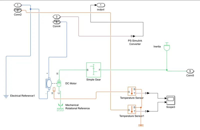
Explanation
- We have connected supply voltage from H bridge to the DC traction motor and motor shaft power is connected to the simple gear input.
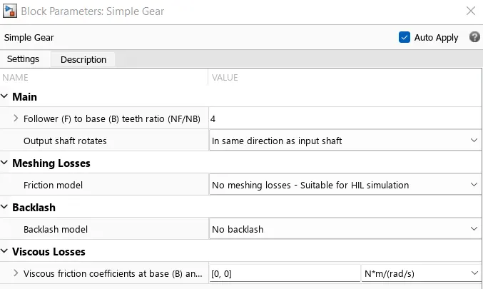
- And output shaft rotates in same direction as input shaft. Mechanical rotational reference is connected to the shaft.
- Two temperature sensors used for monotoring temperature variations of motor and H bridge at different drive cycles.
Traction motor details :
Simple gear details :
Vehicle body subsystem :
Explanation :
- Motor will produce the rotational output which will give to the vehicle body and transmission system. The rotational output is taken by the gear system here to maintain the constant speed throughout the transmission without any loss in speed from the motor to tires.
- Below is a diagram that is how it is how it inside the vehicle body and transmission system and in the main design, it is referred just only as a transmission system.
- Here I created a Rear wheel drive transmission system.
- The gear output is given to axels of Rear tires, in the circuit it is shown that gear is connected to Rear wheels and front tire is free to rotational motion, thus vehicle moves forward. N is the normal force caused by the tires and it is given to the vehicle body normal force port.
- The vehicle body has an H-Hub, S- Tire slip, N- Normal force, A- axel connection, wind velocity, inclination angle. The tires hub is connected as a common node to the vehicle body.
- The vehicle body wind velocity is connected to a constant block and the beta-inclination angle is connected to another constant block where we can assign wind velocity and inclination angle as per requirement. Velocity is the output port where we can get at which speed the vehicle is moving. The velocity is taken out to the get the distance travelled and state of charge.
Battery subsystem
Explanation
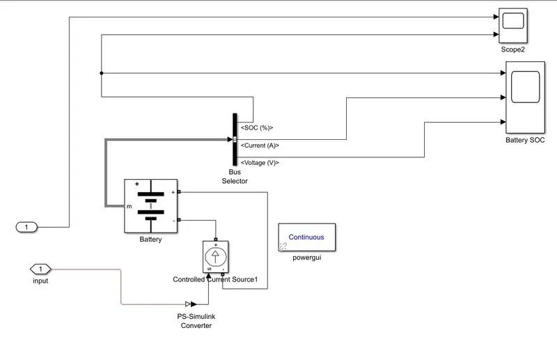
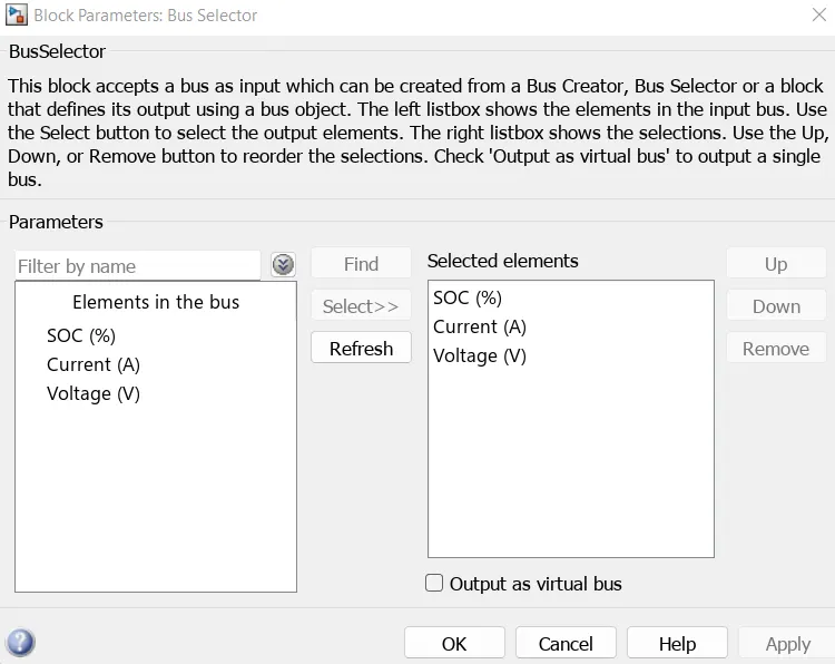
Here we have connected m terminal of battery to bus selector so that we can observe the performance of parameters of battery i.e SOC, Current,Voltage.
- The battery is required to power the controller and motor. The controller uses the battery power according to produce the input given by the motor to obtain maximum speed. The battery is also used to power every electrical component in the vehicle.
- The Battery block implements a generic dynamic model that represents most popular types of rechargeable batteries.
Details of Bus selector :
Details of Battery :
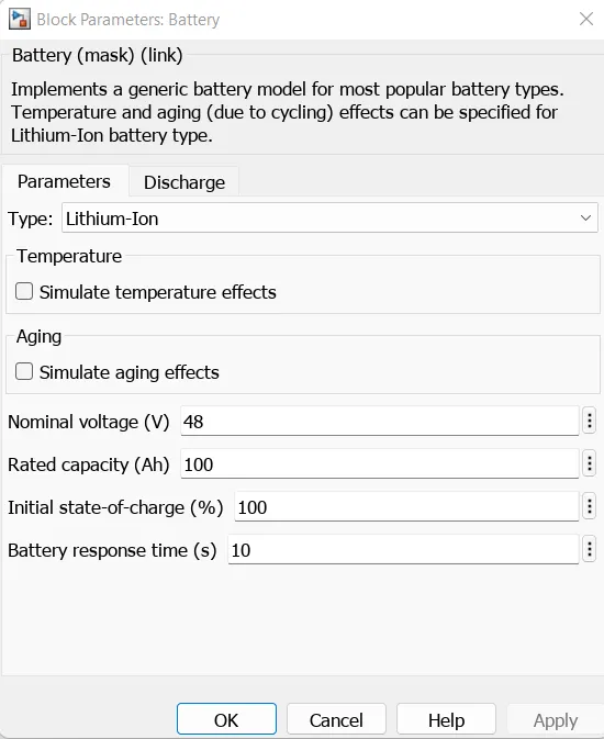
The battery has two stage one is charging and another one is discharging state. The battery is of 100Ah capacity.
The Nominal voltage of battery is 48 V
Initial SoC is of 100%
- where SoC is the state of charge and Vnom is the nominal voltage. Coefficient beta is calculated to satisfy a user-defined data point [AH1,V1].
- The battery has a positive and negative terminal which is given the voltage-controlled source where the battery consumption is controlled by the motor controller and then it is given to the SOC block.
Battery State of Charge :
- SoC is the percentage or level of battery presents after certain travel or consumption of battery charge by the vehicle.
- In the designed vehicle battery charge or SOC is calculated by the giving it to the rate transition and then to gain where 1/(nominal battery capacity) then to a discrete-time integrator and it will get minus from the 1 as it is considered a 100% of battery and it is multiplied with 100 to get percentage of battery.
- The majority of blocks are simscape blocks where physical to simulink converter is used to convert the physical signal from simscape block to simulink signal.
BUS Selector :
- The Bus Selector block outputs the signals you select from the input bus. The block can output the selected elements separately or in a new virtual bus.
- Here just we have mange the output and connect with different Scope Block.
Longitudinal Driver :
- Longitudinal Driver is an inbuilt block provided by the powertrain blockset.
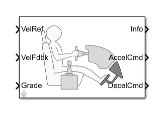
- It is a parametric longitudinal speed tracking controller for generating normalized Acceleration and Braking commands based on reference and feedback velocities.
- The VelFdbk port corresponds to the feedback velocity. The actual velocity output given by the vehicle body is connected here. By comparing the actual (feedback) velocity with the reference velocity, the driver block generates acceleration and braking signals in order to minimise the error between the two concerned velocities.
- Grade corresponds to the grade angle. For this simulation, no inclination is considered and hence, a constant block with value 1 is connected.
- Info gives the output for the bus signal for different block calculations like difference in reference vehicle speed and vehicle speed, etc.
- AccelCmd & DecelCmd correspond to the acceleration and deceleration commands generated respectively and are connected to the corresponding ports of the Controlled PWM Voltage block.
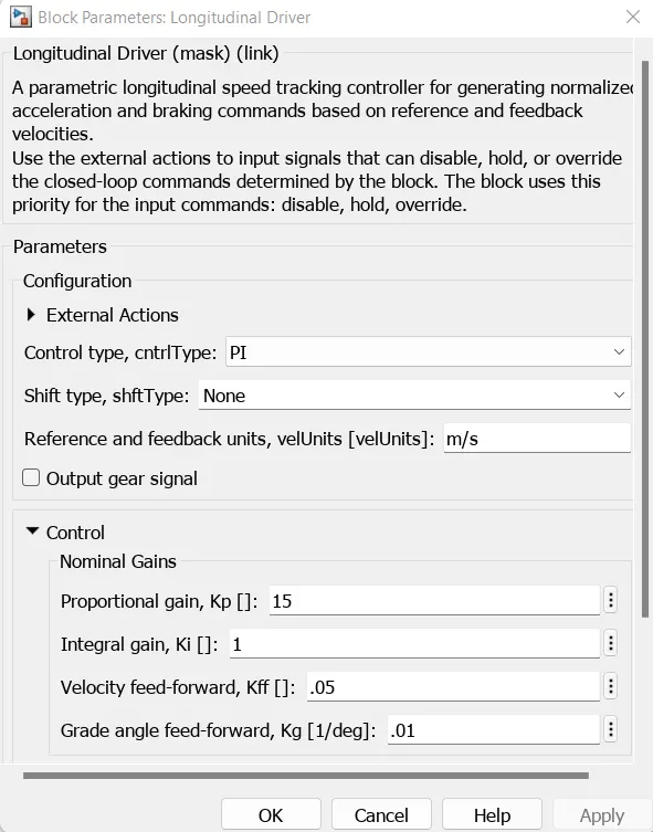
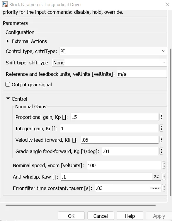
- Here, the selected control type is PI. Acordingly, the block implements proportional-integral (PI) control with tracking windup and feed-forward gains.
Longitudinal driver block details :
H-Bridge :
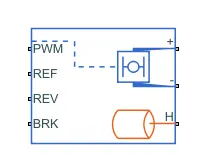
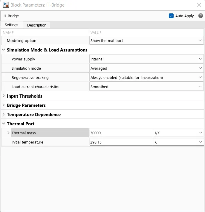
- This block represents an H-bridge motor drive. The block can be driven by the Controlled PWM Voltage block in PWM or Averaged mode. In PWM mode, the motor is powered if the PWM port voltage is above the Enable threshold voltage.
- In Averaged mode, the PWM port voltage divided by the PWM signal amplitude parameter defines the ratio of the on-time to the PWM period. Using this ratio and assumptions about the load, the block applies an average voltage to the load that achieves the correct average load current.
- The Simulation mode parameter value must be the same for the Controlled PWM Voltage and H Bridge blocks.
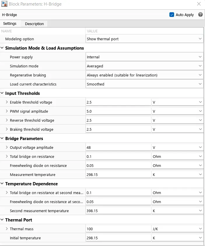
- If the REV port voltage is greater than the Reverse threshold voltage, then the output voltage polarity is reversed. If the BRK port voltage is greater than the Braking threshold voltage, then the output terminals are short circuited via one bridge arm in series with the parallel combination of a second bridge arm and a freewheeling diode.
- Voltages at ports PWM, REV and BRK are defined relative to the REF port. If exposing the power supply connections, the block only supports PWM mode.
Reference Velocity (Drive Cycle) :
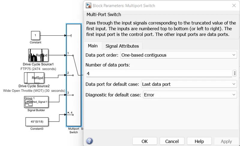
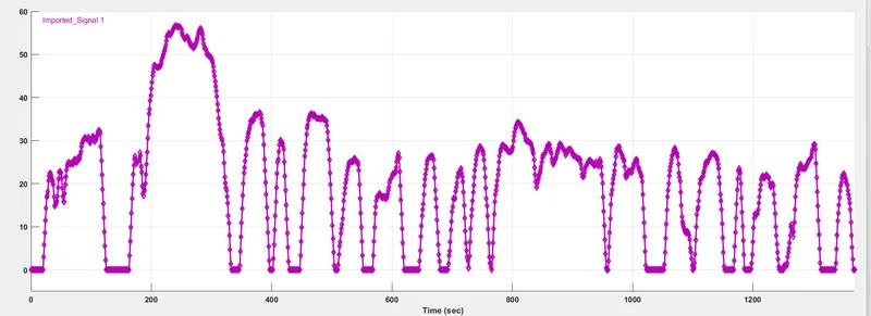
- Drive cycle is assumed as the driver's input of a vehicle, it replaced how a driver will drive a vehicle. Here We have used three drive cycles which is used to test the vehicle performances. These drive cycle will have high speed, low speed, braking conditions in it.
- There are different drive cycles like WOT, FTP75 etc., Here in this model We have used FTP 75, WOT & Manually prepared in excel Drive Cycle source.
- All 3 Drive cycles are controlled by the controller provided above by constant through Multi-port switch.
FTP75
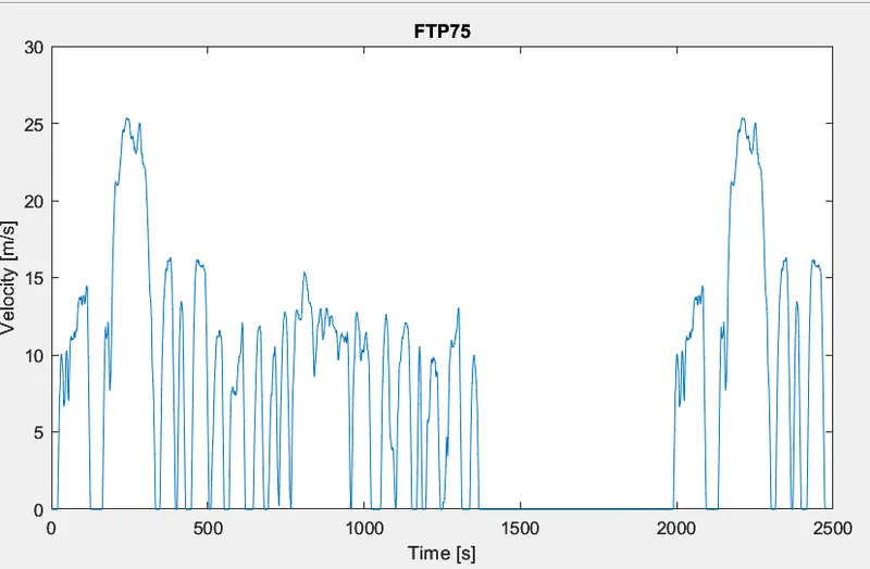
Generates a standard or user-specified longitudinal drive cycle. The block output is the vehicle longitudinal speed. You can import drive cycles from :
- Predefined sources
- Workspace variables, including arrays and time series objects
- mat, xls, xlsx, or txt files
Use the fault tracking parameters to identify drive cycle faults within specified speed and time tolerances.
Wide Open Throttle (WOT) :
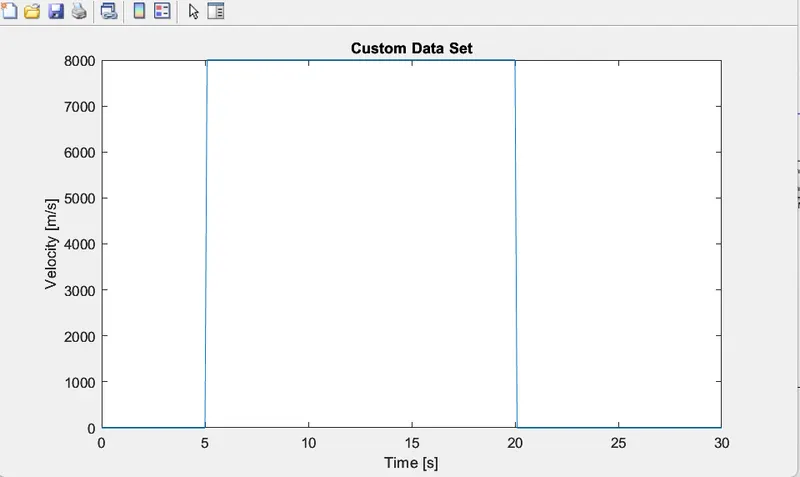
Drive cycle by Signal builder(Manually prepared)
Temperature parameters
1.for H bridge .
2.for DC motor.
Simulink Explanation :
- Initially the current flows to DC Motor from the battery through the DC-DC power converter to drive the motor. The required voltage will be controlled in the controller. The Controller will follow the given drive cycle reference and run the motor in the required rpm.
- Then the motor power is transmitted to the wheels of a vehicle through the gear box. and the controller will take the vehicle speed and compare and controlled.
Output Plots :
For stop time 2745.
1. For FTP75 Drive Cycle :
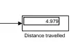
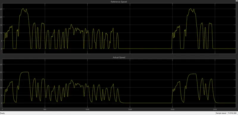
- By running the Vehicle with FTP75 Drive cycle for 2474 sec. the distance travelled is 4.97km.
Reference speed and actual speed
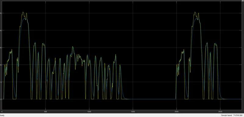
Observation :
- The actual Speed is approximately followed the 90% of reference Drive cycle.
Reference speed and actual speed.
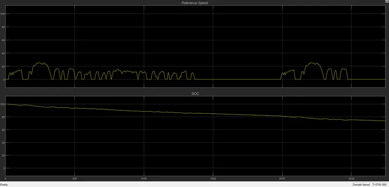
Reference Speed and State of charge (SOC)
SCO,Current and Voltage
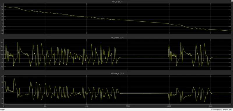
Battery SOC is 100 at initial to 64 at final .
Battery current is 100 at initial to 64 at final.
Battery voltage is 56 at initial to 51 at final.
H Bridge and Motor temperatures.
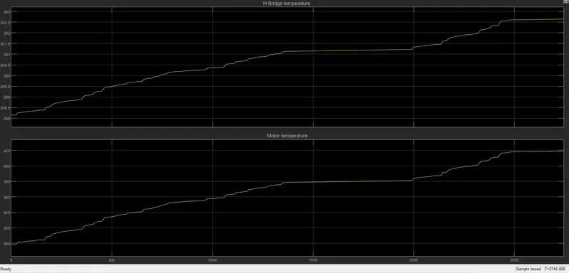
- The temperature of Motor and H bridge is increasing as vehicle moves.
- Temperature parameters of H bridge and motor are little bit constant at time 1400sec to 1900 secs.
- The Temperature of Controller is reached approximately ≈ 303 degree celcious, And motor is 419 degree celcious.
CONCLUSION :
- Here I have compromised with the temperature of Motor and controller to achieve vehicle speed is near to reference speeds. Since We haven’t used any cooling system in the model. In the real time application, the motor temperature is less than 100 C.
- In the real time application, the motor, battery & controller temperature is controlled by air cooling. Hence, the temperature of this components is not increased to this extent.
- Hence, Created a MATLAB model of an Electric Rickshaw (three wheel passenger vehicle) by using Li-ion battery, PM Brushed DC Motor.
- Detremined the variations of Temperature of Motor and controller, SOC% and Energy consumed by the by vehicle for all the three Reference Drive cycles (i.e.; FTP75, WOT, Manually prepared).
- This Battery powered Rickshaw will be the most popular mode of transport in the future.
- We can maintain cooling of controller by using fan or mini chiller plant inside vehicle so that we can improve efficiency of vehicle.