Final Project: Electric Rickshaw modelling

AIM: To create a detailed MATLAB model of an Electric Rickshaw (three-wheel passenger vehicle).

OBJECTIVES:

1. The rear wheels are driven by PM brushed-type motor
2. Assume the efficiency points of the motor controller and motor
3. Make an excel sheet of all input and assumed data
4. Results: For any three standard driving cycles show energy consumption, a temperature rise of motor and controller for 100 km constant speed driving at 45 kmph

THEORY:

About E-Rickshaw

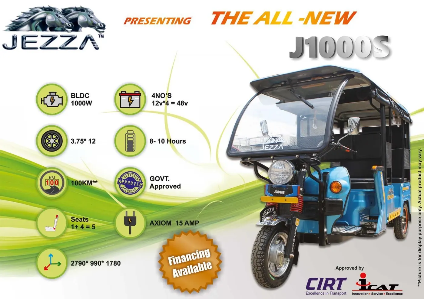
• Electric Rickshaws are small three-wheeled vehicles powered by an electric motor and battery ranging from 650 to 1400 W. They save on fuel costs compared to auto rickshaws while offering greater ease of use than pulled rickshaws. This has increased their popularity and acceptance in some cities since 2008.
  

Design and construction

• These rickshaws have a mild steel tubular chassis, consisting of three wheels with a differential mechanism at the rear wheels. The motor is a Brushless DC (BLDC) motor.
• The electrical system used in Indian versions is 48V and in Bangladesh is 60V. The body design from the most popular Chinese version is of fragile iron or aluminium sheets.
• Bodies made of fibreglass are also popular because of their strength and durability, resulting in low maintenance. The body design is varied from load carriers, and passenger vehicles with no roof, to full-bodied windshields for drivers' comfort.
• It consists of a controller unit. They are sold based on the voltage supplied and current output, also the number of MOSFET (Metal Oxide Field Effect Transistors) used.
• The vehicle's batteries are typically lead acid with a lifespan of 6-12 months. Deep-cycle batteries for electric vehicles are rarely used. The weight of the electric car has also been a recurring design difficulty in them.
• The load-carrying versions of these rickshaws differ in their upper body, load-carrying capacity, motor power, controller and other structural aspects, sometimes motor power is also increased to carry loads up to 500-1000 kg.

Block diagram

Now let us consider a block diagram for the simulation model.

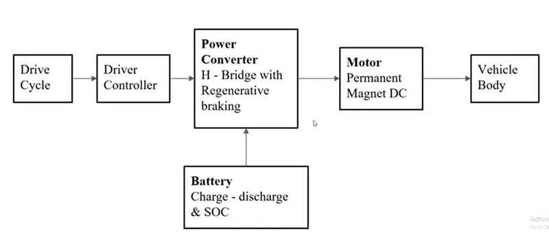
• We will first consider a vehicle body that consists of four axles. Then we will consider a motor and connect it to the axles of the vehicle body.
• The Battery is used for charging the vehicle. If the battery is connected directly to the motor, the motor will run at the rated speed and hence, the vehicle cannot be controlled. So, before connecting the battery directly to the motor, we require a motor controller which changes the speed of the vehicle. This is possible by a power converter, which is an H-bridge with Regenerative braking.
• Now, the battery is supplied to the power converter; the power converter will change the voltage applied to the motor and hence, it will change the vehicle's speed.
• This is the basic block diagram of the electric vehicle. To simulate and run this model for the given input, we need to have a throttle and brake pedal. Therefore, we add a drive cycle that can help us in providing acceleration or deceleration to the vehicle.
• The drive controller tracks the actual speed of the vehicle and matches it with the given input.
  
  

Now let us start the Simulation Model.

SIMULATION MODEL:

i. E-rickshaw Subsystem:

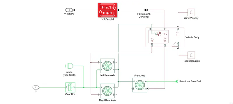
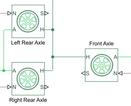
• Since we are modelling an electric rickshaw, we need three tires for the vehicle to run.
  

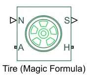
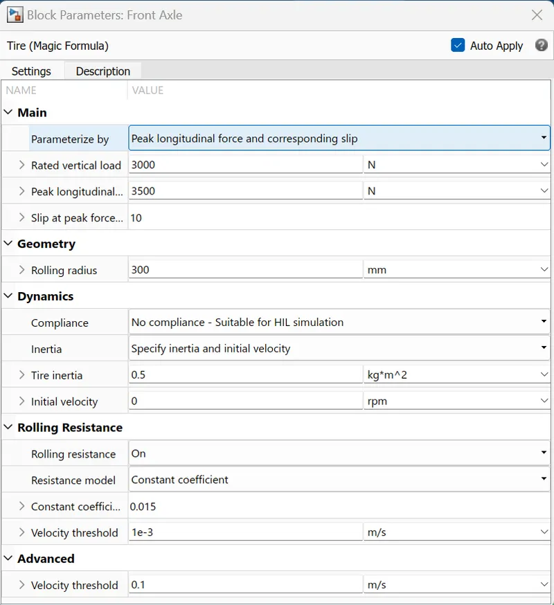
• The Tire (Magic Formula) block represents the longitudinal behaviour of a highway tire characterized by tire Magic Formula. The block is built from Tire-Road Interaction (Magic Formula) and Simscape Foundation Library Wheel and Axle blocks. Optionally, the effects of tire inertia, stiffness, and damping can be included. Connection A is the mechanical rotational conserving port for the wheel axle. Connection H is the mechanical translational conserving port for the wheel hub through which the thrust developed by the tire is applied to the vehicle. Connection N is a physical signal input port that applies the normal force acting on the tire. The force is considered positive if it acts downwards. Connection S is a physical signal output port that reports the tire slip. Optionally expose physical signal port M by setting Parameterize to Physical signal Magic Formula coefficients. Physical signal port M accepts a four-element vector corresponding to the B, C, D, and E Magic Formula coefficients.

• The parameters of the tire are given below:
  
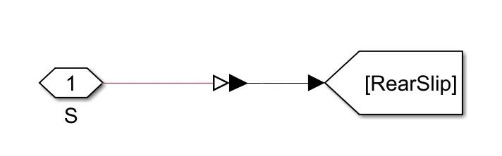
• The S port on the Left Rear Axle and the Left Front Axle tires are modelled with a certain degree of slip using a small subsystem. The slip subsystem used for the tires is shown in the image below.
  
• Now we need a vehicle body to install all these three tyres.
  

• The Vehicle Body block represents a two-axle vehicle body in longitudinal motion. The block accounts for body mass, aerodynamic drag, road incline, and weight distribution between axles due to acceleration and road profile. The vehicle can have the same or a different number of wheels on each axle. Optionally include pitch and suspension dynamics or additional variable mass and inertia. The vehicle does not move vertically relative to the ground. Connection H is the mechanical translational conserving port associated with the horizontal motion of the vehicle body. The resulting traction motion developed by tires should be connected to this port. Connections V, NF, and NR are physical signal output ports for vehicle velocity and front and rear normal wheel forces, respectively. Wheel forces are considered positive if acting downwards. Connections W and beta are physical signal input ports corresponding to headwind speed and road inclination angle, respectively. If a variable mass is modelled, the physical signal input ports CG and M are exposed. CG accepts a two-element vector representing the x and y distance offsets from vehicle CG to additional load mass CG. M represents the additional mass. If both variable mass and pitch dynamics are included, the physical signal port J accepts the inertia of the additional mass about its CG.

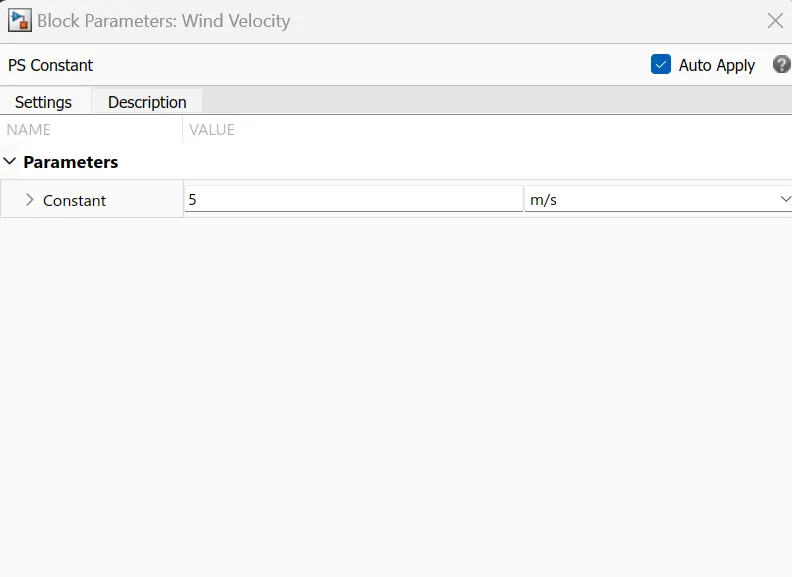
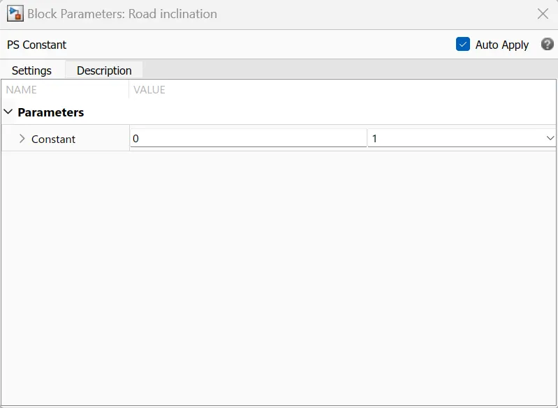
• I modelled the parameters of the W (Wind Velocity) and beta (Road inclination) by adding a PS-Constant block. This block creates a physical signal constantly.
  
  
• Now let us assume that the rear axles are connected to a gear system. So, we'll use a Gear Box.
  

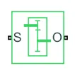
• The Gear Box block represents an ideal, non-planetary, fixed gear ratio gearbox. The gearbox is characterized by its only parameter, Gear ratio, which can be positive or negative. Connections S and O are mechanical rotational conserving ports associated with the box input and output shaft, respectively. The gear ratio is determined as the ratio of the input shaft's angular velocity to that of the output shaft. This block generates torque in the positive direction if a positive torque is applied to the input shaft and the ratio is assigned a positive value.

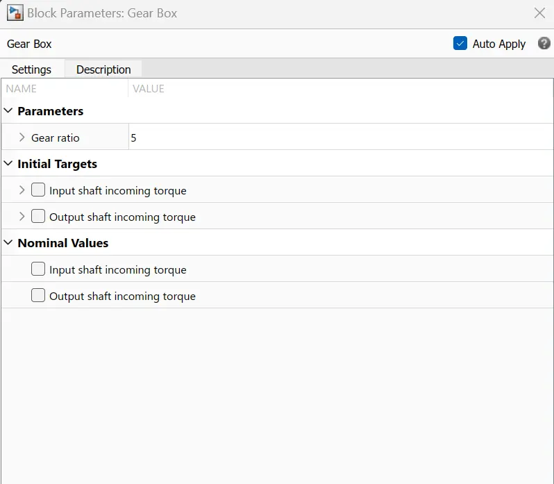
• The parameters of the gearbox are as shown below:
  
• We can also use a side shaft by adding an Inertia block. This block represents an ideal mechanical rotational inertia. This block has one or two mechanical rotational conserving ports. The difference is purely graphical, as the ports are rigidly linked. The block's positive direction is from its port to the reference point. This means that the inertia torque is positive if the inertia is accelerated in the positive direction.
  
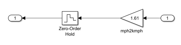
• The mph2kmph subsystem converts the output speed of the vehicle from mph (miles per hour) to kmph (kilometre per hour). The Zero-Order Hold block is used to implement a zero-order hold sample period.
  

ii. DC Motor Drive Subsystem:

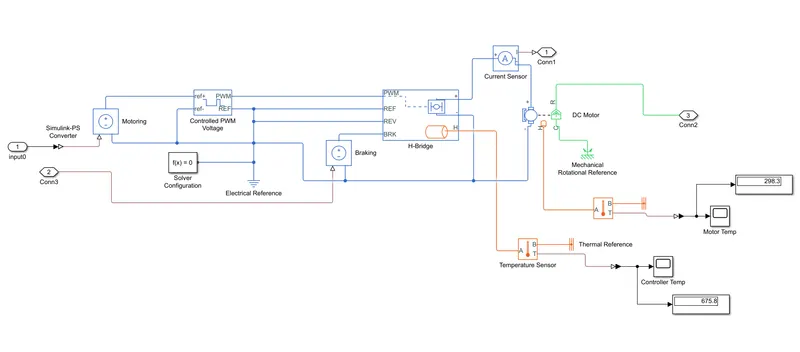
• Now, to run the vehicle, we need an electric motor. So, let us take a simple DC motor block.
  
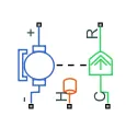
• This block represents the electrical and torque characteristics of a DC motor. The block assumes that no electromagnetic energy is lost, and hence the back-emf and torque constants have the same numerical value when in SI units. Motor parameters can either be specified directly or derived from the no-load speed and stall torque. If no information is available on armature inductance, this parameter can be set to some small non-zero value. When a positive current flows from the electrical + to - ports, a positive torque acts from the mechanical C to R ports. Motor torque direction can be changed by altering the sign of the back-emf or torque constants. The R port of the DC motor is connected to the B port of the simple gear. The C port of the DC motor is connected to the Rotational Reference block.
  
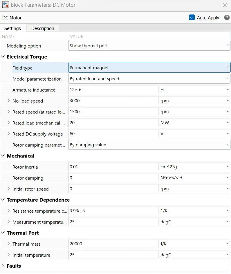
• The DC motor block parameters are changed as shown in the figure below:
  
• Now we need to control the DC motor. It can be done by connecting a DC-DC converter. As mentioned in the block diagram, we can use an H-bridge block.
  
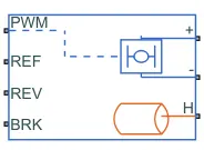
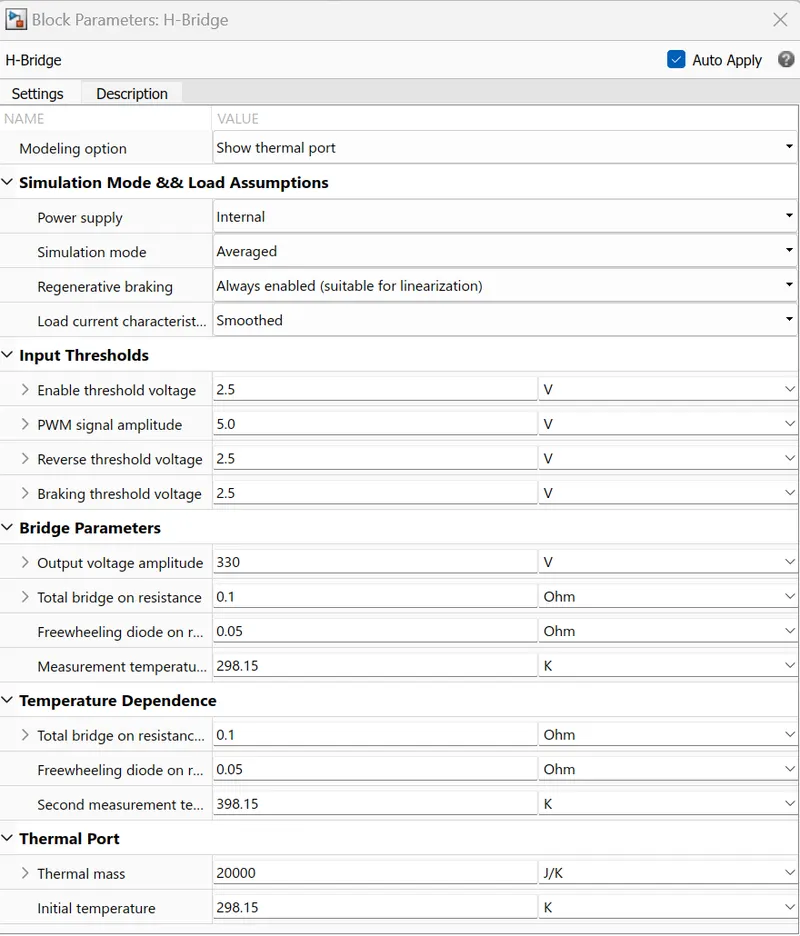
• This block represents an H-bridge motor drive. The block can be driven by the Controlled PWM Voltage block in PWM or Averaged mode. In PWM mode, the motor is powered if the PWM port voltage is above the Enable threshold voltage. In an Averaged manner, the PWM port voltage divided by the PWM signal amplitude parameter defines the ratio of the on-time to the PWM period. Using this ratio and assumptions about the load, the block applies an average voltage to the load that achieves the correct average load current. The Simulation mode parameter value must be the same for the Controlled PWM Voltage and H-Bridge blocks.
• If the REV port voltage exceeds the Reverse threshold voltage, then the output voltage polarity is reversed. Suppose the BRK port voltage is greater than the Braking threshold voltage. In that case, the output terminals are short-circuited via one bridge arm in series with the parallel combination of a second bridge arm and a freewheeling diode. Voltages at ports PWM, REV and BRK are defined relative to the REF port. If exposing the power supply connections, the block only supports PWM mode.
• The block parameters are changed as shown in the figure below:
  
• Now we need to control the Pulse Width Modulation. For that, we can use the Controlled PWM Voltage block.
  
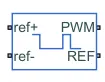
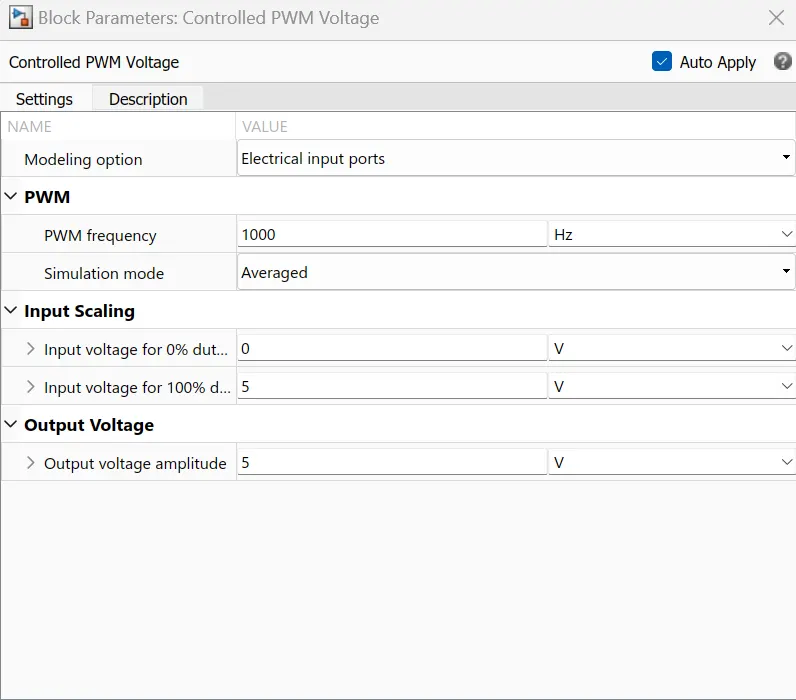
• This block creates a Pulse-Width Modulated (PWM) voltage across the PWM and REF ports. The output voltage is zero when the pulse is low and is equal to the Output voltage amplitude parameter when high. The duty cycle is set by the input value. At time zero, the pulse is initialized as high unless the duty cycle is set to zero or the Pulse delay time is more significant than zero. The Simulation mode can be set to PWM or Averaged. In PWM mode, the output is a PWM signal. In Averaged mode, the output is constant with a value equal to the averaged PWM signal.
• The block parameters are as shown below:
  
• Now let us not explore the REV port in the H-Bridge block. So, we'll connect it to the Electrical Reference Block.
  
• Now the PWM voltage can be controlled only when there is an input. So, we'll add a Controlled Voltage Source block. This block represents an ideal voltage source powerful enough to maintain the specified voltage at its output regardless of the current passing through it. The output voltage is V = Vs, where Vs is the numerical value presented at the physical signal port.
• But that will be only for motoring mode. We'll add another block for braking mode to the BRK port of the H-bridge.
• The Solver Configuration block defines solver settings to use for simulation.
  
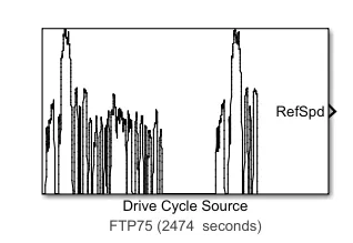
• To run our vehicle, we need an input source to start the vehicle. Hence, we'll use a Drive Cycle Source block.

  The Drive Cycle Source block generates a standard or user-specified longitudinal drive cycle. The block output is the specified vehicle longitudinal speed, which you can use to:

  • Predict the engine torque and fuel consumption that a vehicle requires to achieve desired speed and acceleration for a given gear shift reference.

  • Produce realistic velocity and shift references for closed-loop acceleration and braking commands for vehicle control and plant models.

  • Study, tune, and optimize vehicle control, system performance, and system robustness over multiple drive cycles.

  • Identify the faults within tolerances specified by standardized tests, including:

    • EPA dynamometer driving schedules.

    • Worldwide Harmonised Light Vehicle Test Procedure (WLTP) laboratory tests.

    
    

• Now to convert this velocity into an Acceleration/Deceleration Command, we'll use a Longitudinal Driver block. This block is a parametric longitudinal speed tracking controller for generating normalized acceleration and braking commands based on reference and feedback velocities.
  

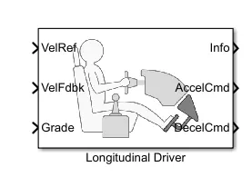
• The Drive Cycle source is connected as a reference to the VelRef port of the Longitudinal Driver. This means that the driver is constantly following the vehicle's reference speed and it will compare it with the vehicle's feedback speed coming from the Electric Car. If there is any positive error i.e. VelRef > VelFdbk, then the driver is going to press the accelerator (AccelCmd). If VelFdbk > VelRef, then the driver is going to press the brakes (DecelCmd).
• We'll use the Simulink-PS Converter block to add the AccelCmd & DecelCmd to the respective Controlled Voltage Sources. This block converts the Simulink input signal to a Physical Signal.

• Similarly, the PS-Simulink Converter block converts the Physical input Signal to a Simulink output signal.

iii. Battery Subsystem:

• Now, we have created the input to run the vehicle. Now, we need to run the DC motor, which is possible by adding a Battery block. This block models a battery. If you select Infinite for the Battery charge capacity parameter, the block models the battery as a series of internal resistance and a constant voltage source. If you select Finite for the Battery charge capacity parameter, the block models the battery as a series of internal resistance plus a charge-dependent voltage source defined by:

  V = Vnom*SOC/(1-beta*(1-SOC))

  where SOC is the state of charge and Vnom is the nominal voltage.
  

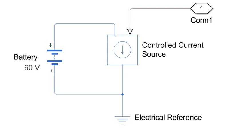
• The Controlled Current Source block represents an ideal current source that is powerful enough to maintain the specified current through it regardless of the voltage across it.
• Now, I may need to have an emitter in between the battery and the H-bridge to measure the current taken by the motor. So, I can measure this current by adding a Current Sensor block. This block represents an ideal current sensor, that is, a device that converts current measured in any electrical branch into a physical signal proportional to the current. Connections + and - are conserving electrical ports through which the sensor is inserted into the circuit. Connection I is a physical signal port that outputs the current value.
  

iv. SOC Calculation Subsystem:

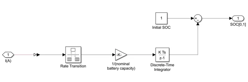
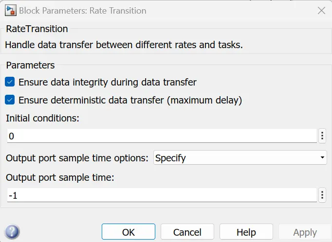
• The Rate Transition block handles data transfer between different rates and tasks.

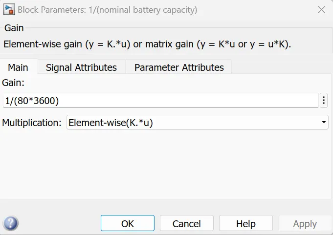
• The Gain block provides the formula for SOC calculation.

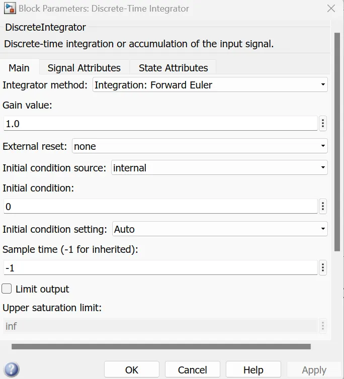
• The Discrete-Time Integrator block is used to perform a discrete integration of the current signal concerning the time.

• A Constant block is used to represent the initial SOC of the battery. Assuming that the battery is always fully charged when performing a simulation, I have altered the constant block with a value of 1 representing 100%.
• The Sum block is used to perform addition and subtraction operations. The signal from the Discrete-Time integrator block will be subtracted from the constant block representing 100% charge.

v. Output:

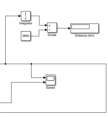
• The Integrator block is used to integrate the output velocity concerning time to give us the distance travelled.
• The Divide block is used to divide the integrated speed signal which is in kmph by a constant block valued at 3600. This will give us the distance in km.

RESULT:

• The below figure shows us the entire simulation model of the Electric Rickshaw.
  
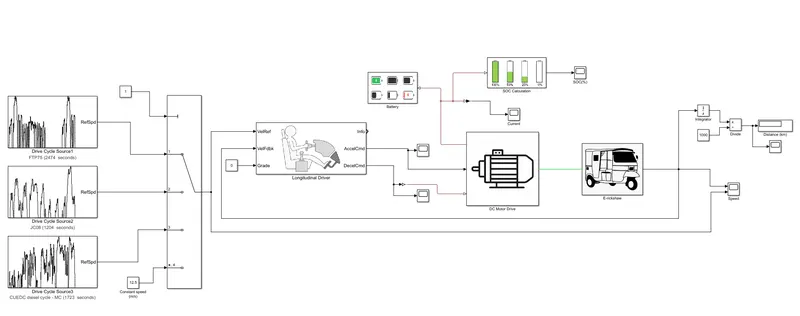
• The Simulation time should be set to the time given in the Drive Cycle Source. For eg., if the time given in the FTP-75 Drive Cycle is 2474 seconds, the simulation time should be set to 2474 seconds. Similarly, if the time given in the WOT drive cycle is 30 seconds, the simulation time should be set to 30 seconds.
• In this model, I've chosen three input drive cycle sources FTP-75, JC08 & CEUDC and the simulation time is set to them.

The outputs (or scopes) of the Simulation Model are as shown below:

i. Speed

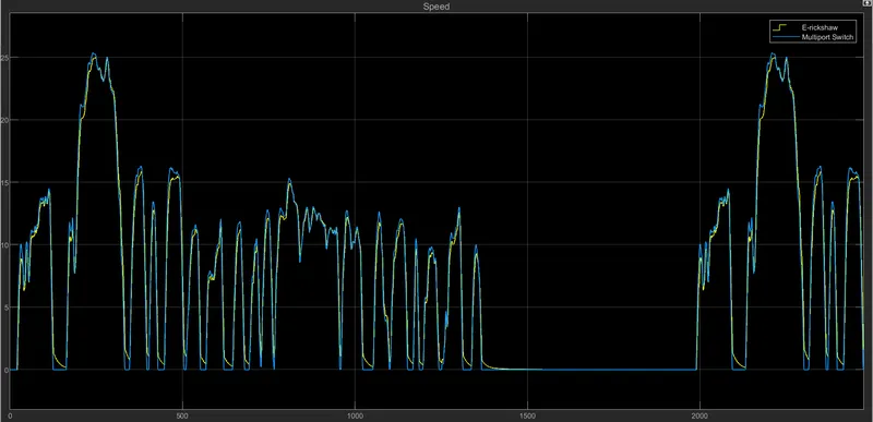
FTP-75 Drive Cycle

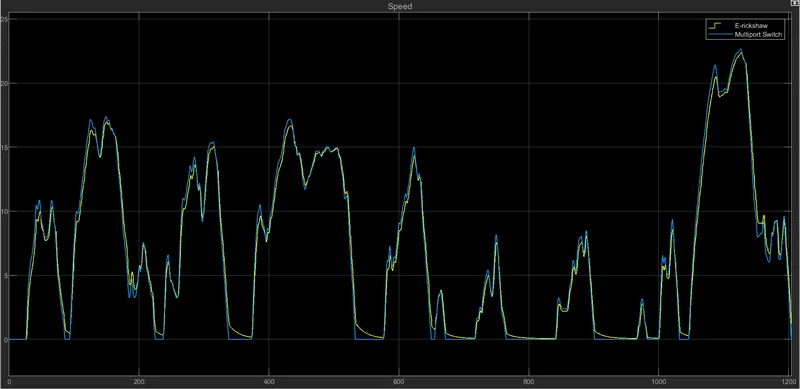
JC08 Drive Cycle

CUEDC Diesel Cycle - MC

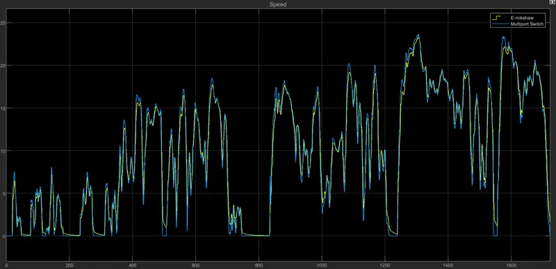
From these scopes, we have 2 signals. The blue signal refers to the Drive Cycle Source and the yellow signal refers to the Vehicle speed. We can observe that the vehicle speed approximately matches the drive cycle speed. This shows that the vehicle is running in good condition.

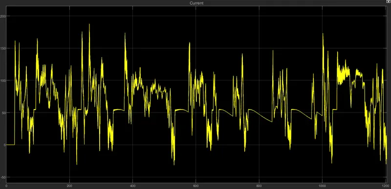
ii. Battery Current

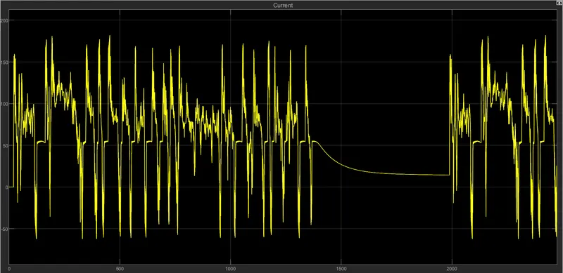
FTP-75 Drive Cycle

JC08 Drive Cycle

CUEDC Diesel Cycle - MC

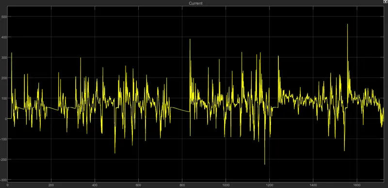
The figures show how the current flowing from the battery to the motor varies concerning the drive cycle time. We can observe that the current is flowing maximum from 0 after a few seconds (say 5 seconds). This means that the maximum current is always required when the car is accelerating from rest due to the inertia of the vehicle. But once the vehicle is in motion, it requires significantly lesser energy to continue accelerating. After some time (say 100 seconds), we can observe that the current instantaneously drops to the negative value (-100 A). This is occurred due to regenerative braking. When the vehicle decelerates, the throttle is no longer applied and so the kinetic energy from the motion is converted to electrical energy fed back to the battery of the EV. This reverse flow causes negative current measurements. However, as the vehicle decelerates, there was lesser energy available for regenerative braking causing the magnitude of the current to decrease. Hence, the polarity of the current moves towards the positive direction because regenerative braking happens lesser and lesser until the vehicle comes to rest.

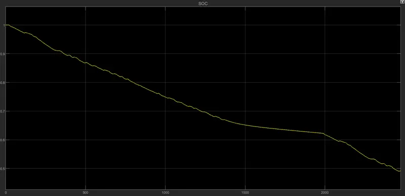
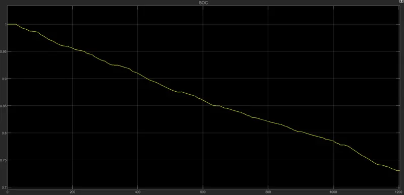
iii. SOC

FTP-75 Drive Cycle

JC08 Drive Cycle

CUEDC Diesel Cycle - MC

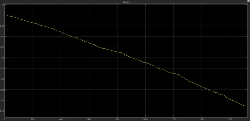
These scopes show us how the state of charge varies over the drive cycle time. When the vehicle is at rest, the SOC of the battery is 1 i.e. 100%. This is because the drive cycles command the vehicle to be at rest for that duration and so no discharge occurs from the battery. When the vehicle begins to accelerate, the SOC of the battery decreases. We can see that the magnitude of SOC increases in between the simulation. This is due to regenerative braking. This effect charges the battery and as a result, increases the SOC of the battery during the deceleration period.

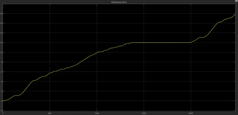
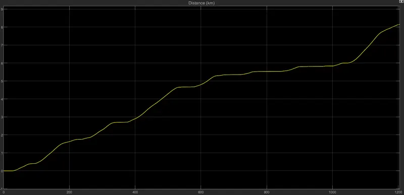
iv. Distance measurement

FTP-75 Drive Cycle

JC08 Drive Cycle

CUEDC Diesel Cycle - MC

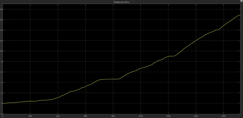
From the images above, we can see that the Display block has measured the distance travelled by the vehicle and the Scope block shows its waveform. The area under the velocity time graph tells us the displacement of an object. So, from looking at the speed scope, the calculation indicates that this distance measurement is correct and accurate.

v. Motor Temperature

FTP-75 Drive Cycle

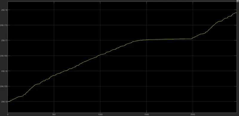
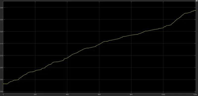
Motor temperature is increased by 100 deg. K when in operation. This temperature rise is very high and needs to be controlled. It can be concluded that a cooling medium is necessary for this powertrain for efficient working and durability.

JC08 Drive Cycle

CUEDC Diesel Cycle - MC

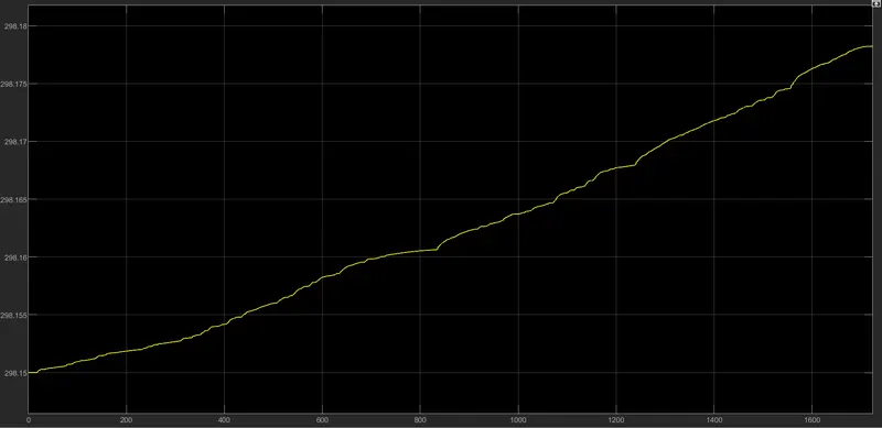
Motor temperature is increased by 100 deg. K when in operation. This temperature rise is very high and needs to be controlled. It can be concluded that a cooling medium is necessary for this powertrain for efficient working and durability.

vi. Controller Temperature

FTP-75 Drive Cycle

JC08 Drive Cycle

CUEDC Diesel Cycle - MC

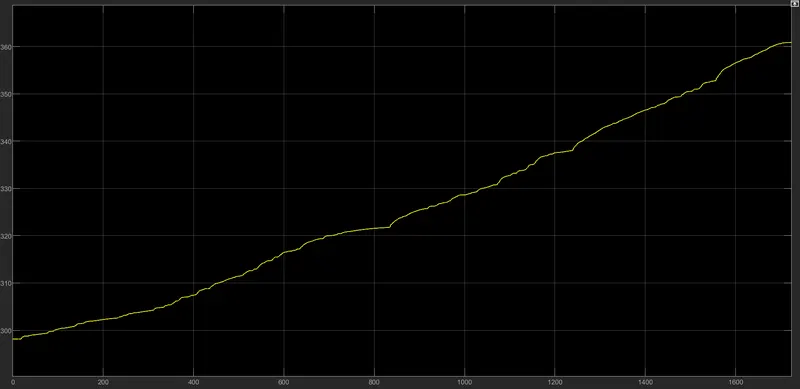
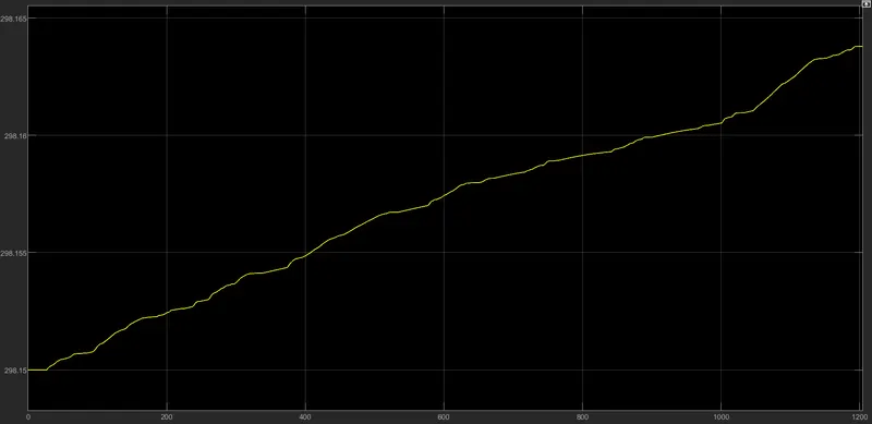
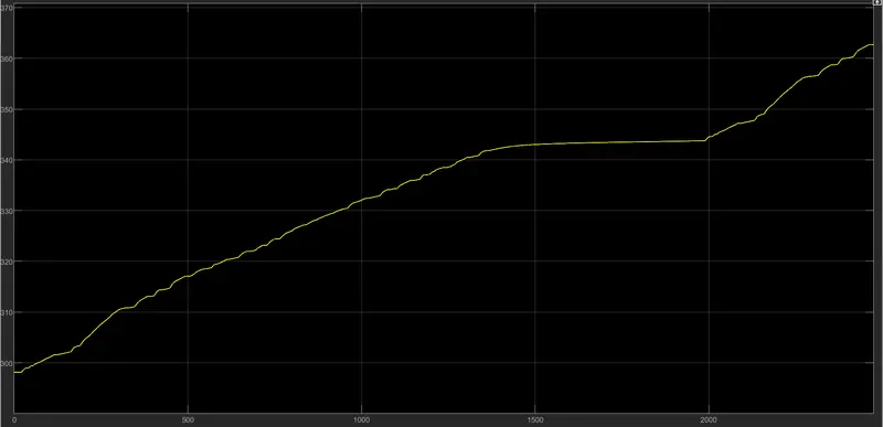
The temperature of the controller rises when the vehicle is running and is constant when it stops. The temperature rise is negligible.

vii. For 100 km running at a constant speed of 45 kmph

Speed

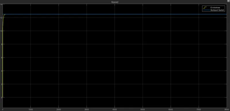
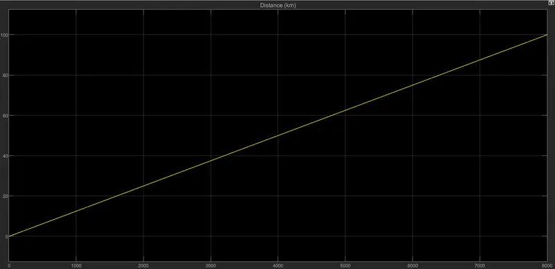
The above plot describes the control accuracy of the system. Input speed and output speed is very identical, meaning the controller is performing its function accurately. The constant speed of 45 kmph (12.5 m/s) is achieved throughout the 100 km distance.

Motor Temperature

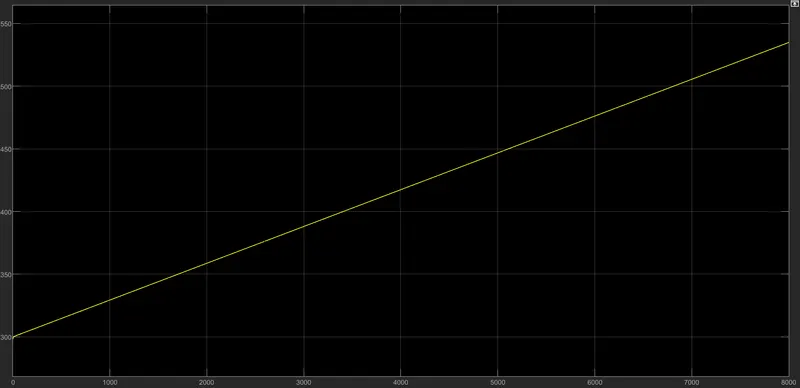
For 0 to 45kmph acceleration, the temperature rise was 298.2 K. As the vehicle completed the 100 km distance, the motor temperature reached 534.8 K.

Controller Temperature

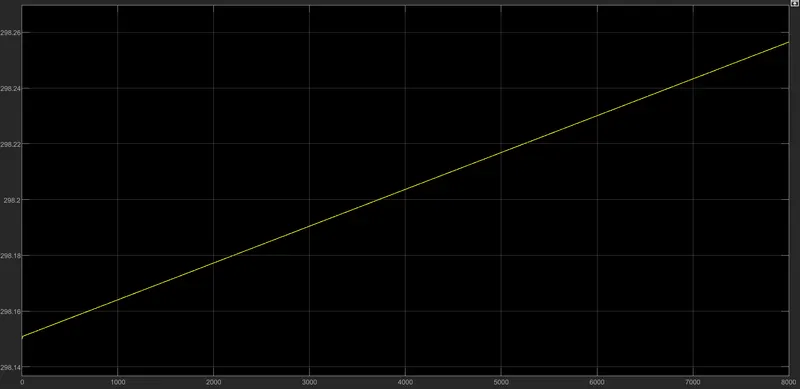
During the 100km travel of the vehicle at a constant 45 kmph speed, the controller temperature has risen from 298.15 to 298.161 K. There is a negligible rise in the controller temperature.

Distance

CONCLUSION:

• I can conclude that the Electric Rickshaw model has been created with the necessary block components using the SIMULINK and the model has been simulated for 3 different drive cycles i.e., FTP-75, JC08 & CUEDC Diesel Cycle.
• The simulation has produced the results of the velocity of the vehicle, the current flowing from the battery, the SOC of the battery, the motor & controller temperature and the distance travelled by the E-rickshaw.
• Since the E-rickshaw model was parameterized to simulate averaged voltage pulses in the H-bridge and Controlled PWM voltage blocks to be fed into the DC motor, the simulation was run very quickly.