Final Project: Electric Rickshaw modelling

Create a detailed MATLAB model of an electric rickshaw (three wheel passenger vehicle) as per details below:

Rear wheels driven by PM brushed type motor

Assume efficiency points of motor controller and motor

Make an excel sheet of all input and assumed data

Results: For any three standard driving cycles show energy consumption, temperature rise of motor and controller for 100 km constant speed driving at 45 kmph.

Solution:

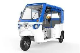
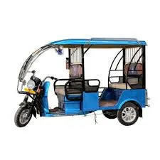
Fig: Electric rickshaw images in different designs. Left (typically called "Auto" in India - D+3 seater),Right(E-rickshaw - D+4 seater)

there are many models available in the E-Rickshaw market and since we have to assume some of the parameters for our model let us take a look at some of the existing E-Rickshaw models in the market and dive deeper into their specifications.

Most of the E-Rickshaws have a speed limit around 25km/hr due to government regulations.(which we will see soon as we look at the models in the market). The motor usually has a size of 1kW and is BLDC in nature. and the operating voltage is aroun 48V.

Consider the following examples:

1) Mini Metro E-rickshaw

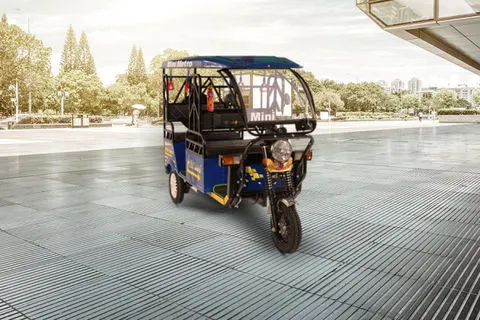
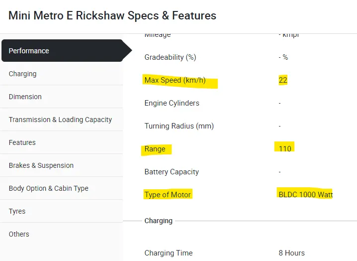
Fig: Mini Metro E rickshaw specs

Fig: Battery specs

2) GEM EV Prince

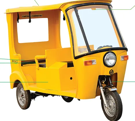
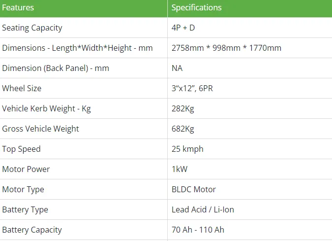
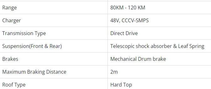
Fig: technical specifications of the Prince model

3) Mahindra Autos(Treo HRT, Trea SFT) and E-Ricksaws(Yaari SFT, Yaari HRT)\

Fig: Mahindra Treo and Treo Yaari

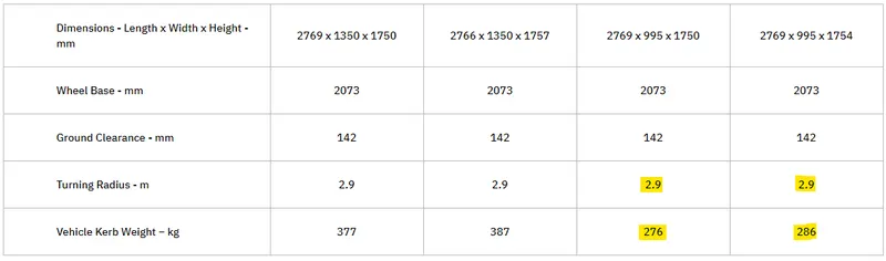
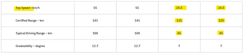
Fig: Specifications of Auto and E-rickshaw by Mahindra Treo Series

4) Zeniak Innovations E-Rickshaw

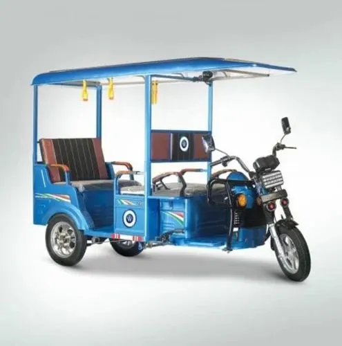
Fig: Zeniak Innovation E rickshaw specs

From the above examples we can see that there is a general range of specifications in E-Rickshaws in the market.

So using these as a general idea we can assume the specification data as follows:

Kerb Weight	190 kg
Maximum load capacity	400 kg
Tyre size marking	90/90-12
Tyre radius (m)	3.7 m
DC motor rated power	1.5 kW
Battery Voltage	48 V
Drag Coefficient	0.55
Frontal area (`m^2`)	1.6

we also need DC motor specifications :

consider the example below

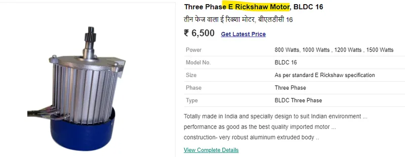
Fig: consider the BLDC type motor for E-Rickshaw. We can use similar rating for our Brushed type motor

Fig: Speed-Torque characteristics of PMDC motor

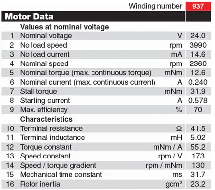
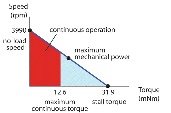
Fig: an example of the PMDC motor operating charateristics and parametric values

so we can take the above characteristics as a reference to model the behavior of our motor. So we maximum conitnuous torque is in the region of about `2/3` of the no load speed.

keeping all this in mind we will create the model and sepcify the ratings of the components for the E-Rickshaw:

First we shall see the component blocks that are required to buid the complete model in detail and the different configurations within them for choosing the appropriate ones for our system model.

Mechanical Components/Subsystems:

Vehicle Body:

Two-axle vehicle with longitudinal dynamics and motion and adjustable mass, geometry, and drag properties

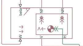
Fig: Vehicle Body Block

It represents a 2 axle vehicle in longitudinal motion. Can have a same or different number of wheels on each axle. Wheels are assumed to be identical in size. Centre of Gravity can be at or below the plane of travel.

The block accounts for:

• Body mass/payload
• Drag coefficient(aerodynamic drag)
• Road inclination(grade)
• Weight distribution on the 2 axles due to acceleration and grade profile
• Has optional pitch & suspension dynamics.

The vehicle does not move vertically relative to the ground.

The block has an option to include an externally-defined mass and an externally-defined inertia. The mass, inertia, and center of gravity of the vehicle body can vary over the course of simulation in response to system changes.

Model axes:The vehicle axles are parallel and form a plane. The longitudinal, x, direction lies in this plane and perpendicular to the axles. If the vehicle is traveling on an incline slope, β, the normal, z, direction is not parallel to gravity but is always perpendicular to the axle-longitudinal plane.

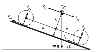
Fig: vehicle dynamics and model variables

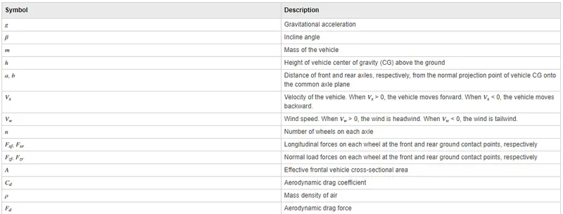
Fig: variables of the Vehicle Body mathematical model

Equations:

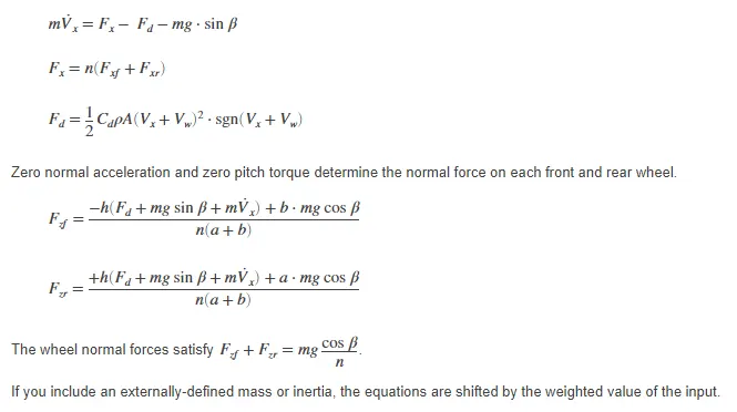
Limitations & Assumptions:

• Only models Longitudinal dynamics,, parallel to the ground and oriented along the direction of motion
• assumed to be in pitch and normal equilibrium. The block does not model pitch or vertical movement
• the equations assume that the wheels never lose contact. This constraint can result in negative normal forces.

Ports:

• W(Wind) - for headwind speed
• Beta - road incline angle
• V - output - longitudinal velocity
• NF - front axle normal force. Wheel forces Considered positive if acting downwards
• NR - Rear axle normal force
• H- horizontal motion - Conserving port associated with the horizontal motion of the vehicle body. Connect tire traction motion to this port.

Block parameters: Main

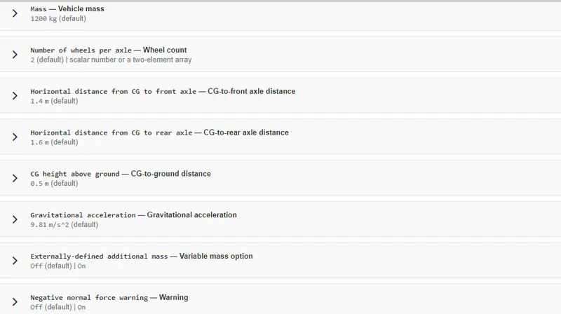
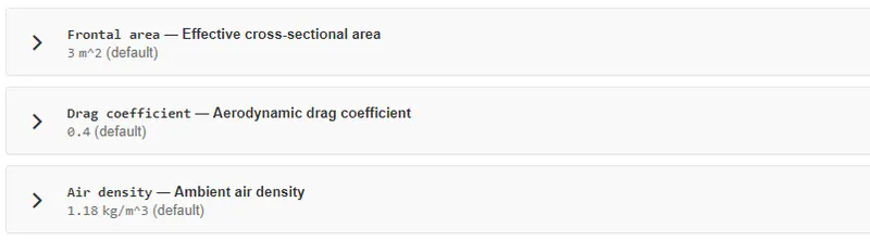
Block parameters: Drag

Block parameters: Pitch

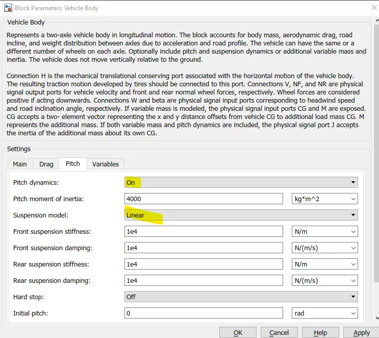
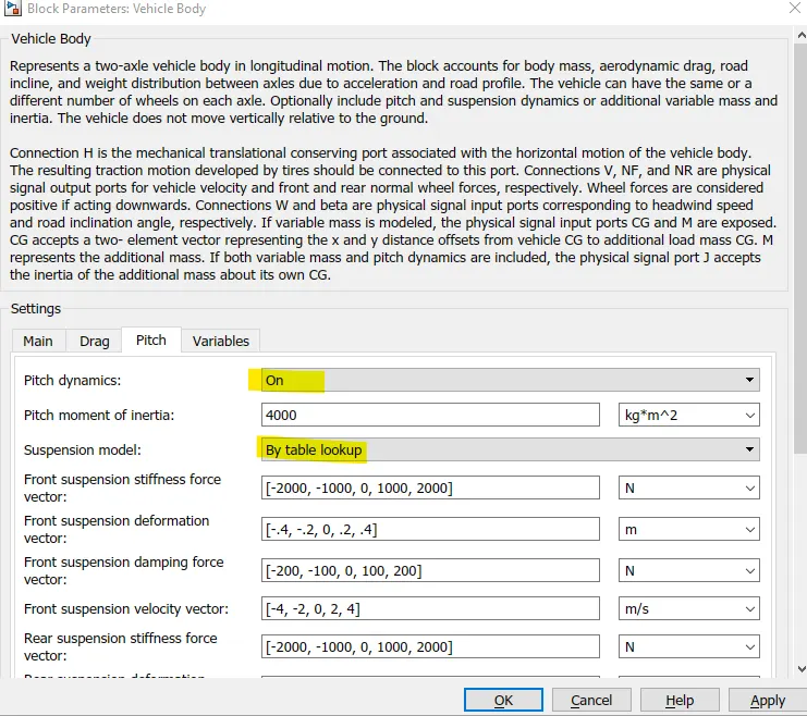
Fig: Pitch parameters if ON then the options under the 2 cases of Suspension model - Linear or Lookup table. Default is OFF

If set to ON- it helps us to Enable Pitch Dynamics Modeling: which needs 3 parameters/dependencies:

1. Suspension model(as we see above image for the 2 types- Linear or Lookup table)
2. Hard-Stop Model
3. Initial Pitch conditions

Last two are also in the same dialog box drop down menu of Pitch :

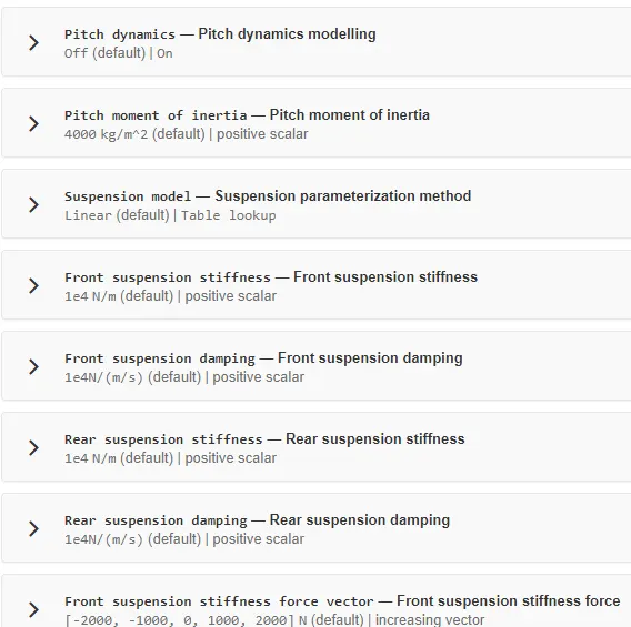
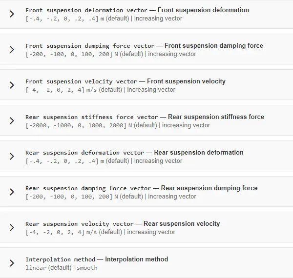
Fig: Some variables that need to be defined for Pitch Dynamic modelling if enabled ‘Pitch’

Tire(Magic Formula):

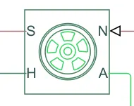
Fig: Tire(Simscape > Driveline) block

Description: For Longitudinal behavior guven by Magic Formula Coefficients, which is an empirical equation based on four fitting coefficients. The block can model tire dynamics under constant or variable pavement conditions.The longitudinal direction of the tire is the same as its direction of motion as it rolls on pavement.

To increase the fidelity of the tire model: you can specify properties such as tire compliance, inertia, and rolling resistance.Tradeoff - these properties increase the complexity of the tire model and can slow down simulation. Consider ignoring tire compliance and inertia if simulating the model in real time or if preparing the model for hardware-in-the-loop (HIL) simulation.

Tire Model:

models the tire as a rigid wheel-tire combination in contact with the road and subject to slip. When torque is applied to the wheel axle, the tire pushes on the ground (while subject to contact friction) and transfers the resulting reaction as a force back on the wheel. This action pushes the wheel forward or backward. (If you include the optional tire compliance, the tire also flexibly deforms under load.)

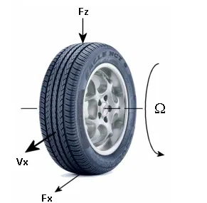
Fig: Forces acting on the Tire (FBD)

Model Variables are as follows:

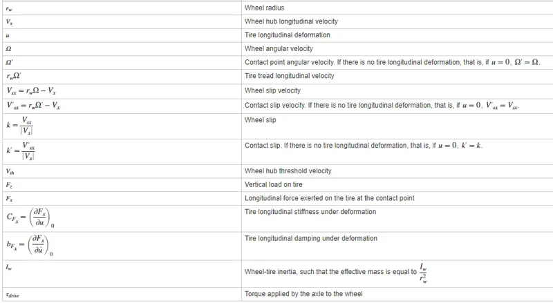
Tire kinematics and Response:

Roll and Slip:

Slip at Low Speeds:

Defromation:

tire and wheel dynamics:

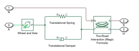
fig: behavior of the block is same as the behavior of the system above

the tire model is equivalent to the above component diagram , simulates both steady state and transient behavior well and correctly represents the staring and coming to stop. Spring and damper are equivalent to tire stiffness and damping due to deformation in the Tire block - refer to variables in the table `C_"F_x"` and `B_"F_x"`

The Tire-Road Interaction (Magic Formula) block models the longitudinal force `F_x` n the tire as a function of `F_z` and `k'` using the Magic Formula, with `k'` as the independent slip variable.

The Wheel and Axle radius is the wheel radius `r_omega`. The Mass value is the effective mass, `I_omega/r_omega^2 ` The tire characteristic functionf(k′,Fz)">f(k',Fz)�(�′,��) determines the longitudinal force Fx">Fx��. Together with the driveshaft torque applied to the wheel axis,Fx">Fx��determines the wheel angular motion and longitudinal motion.

Assumptions and Limitations:

• The Tire (Magic Formula) block assumes longitudinal motion only and includes no camber, turning, or lateral motion.
• Tire compliance implies a time lag in the tire response to the forces on it. Time lag simulation increases model fidelity but reduces simulation performance

Input ports :

• N - Nomal Force: the normal force acting on the tire. The normal force is positive if it acts downward on the tire, pressing it against the pavement.
• M - Magic formula coefficients(only if parameterize by Physical signal Magic Formula coefficients is selected): a four-element vector, specified in the order [B, C, D, E].

Output ports :

• S - Slip - slip between the tyre and the road

Conserving ports :

• A- Axle : Mechanical rotational port associated with the axle that the tire sits on.
• H- Hub: Mechanical translational port associated with the wheel hub that transmits the thrust generated by the tire to the remainder of the vehicle.

Parameters : Main:

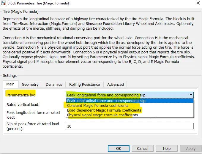
Fig: options to parameterize according to which other parametes will be available

for chosing the Magic formula tire-road interaction model.

The Magic Formula is a specific form for the tire characteristic function, characterized by four dimensionless coefficients, B, C, D, and E, or stiffness, shape, peak, and curvature:

The slope of f at

Magic formula coeffiemts for typical road conditions:

To model under constant pavement condition chose either of:

• Peak longitudinal force and corresponding slip — Parameterize the Magic Formula with physical characteristics of the tire.
• Constant Magic Formula coefficients — Specify the parameters that define the constant B, C, D, and E coefficients as scalars, with these default values.
• Load-dependent Magic Formula coefficients — Specify the parameters that define the load-dependent C, D, E, K, H, and V coefficients as vectors, one for each coefficient, with the default values available in documentation.

To model tire dynamics under variable pavement conditions, select Physical signal Magic Formula coefficients. Selecting this model exposes a physical signal port M. Use the port to input the Magic Formula coefficients as a four-element vector, specified in the order [B, C, D,E].

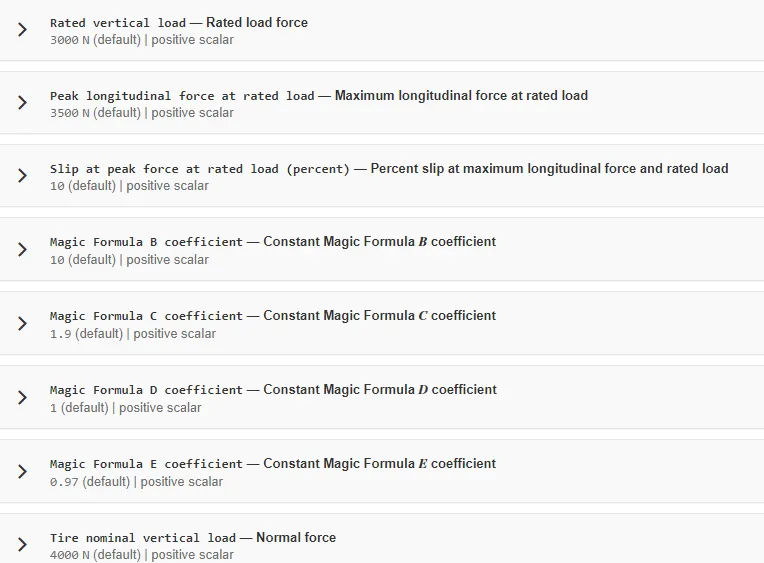
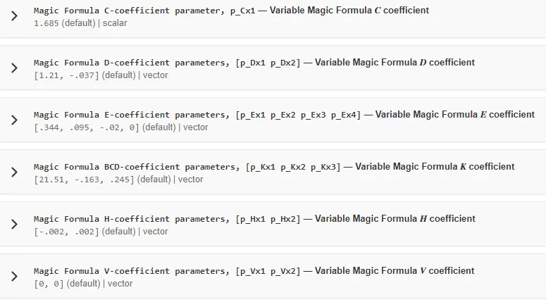
Fig: Parameters(dependent on the choice of 'parameterize by') defined

Geometry:

• Rolling Radius: unloaded tire-wheel radius

Dynamics:

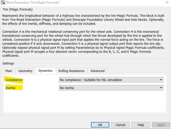
Fig: As before , for incorporating the deformation parameters, but at cost of increased time for simulation (can see No compliance - written as an option "sutiable for HIL" and real time simulation.)

Rolling Resistance: Default OFF:

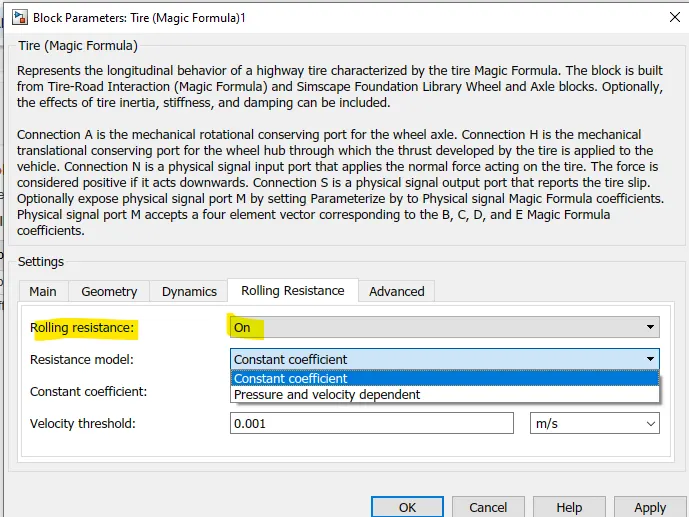
Fig: if ON has 2 options - constant coefficients and Pressure and Velocity dependent

Advanced :

Velocity threshold:Wheel hub velocity `V_"th" ` below which the slip calculation is modified to avoid singular evolution at zero velocity. Must be positive. Refer to equations above to understand significance.

Simple Gear:

Simple gear of base and follower wheels with adjustable gear ratio, friction losses, and triggered faults.

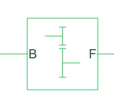
Fig: Simple Gear (Simscape> Driveline)

Description: The Simple Gear block represents a gearbox that constrains the connected driveline axes of the base gear, B, and the follower gear, F, to corotate with a fixed ratio that you specify. You choose whether the follower axis rotates in the same or opposite direction as the base axis.

The kinematic constraint that the Simple Gear block imposes on the two connected axes is:

`=>r_f omega_f = r_b omega_b`

The follower-base gear ratio is

`=>g_"FB" = r_f/r_b = N_F/N_B`

where :

`N_F`= is the number of teeth in the follower gear.

`N_B`= is the number of teeth in the base gear.

Example- Say gear ratio between follower and base is 2:1, then it means that The follower shaft torque is twice the base shaft torque and the angular velocity of the follower is half the angular velocity of the base

Reducing the two degrees of freedom to one independent degree of freedom yields the torque transfer equation:

`=>g_"FB" tau_B + tau_F - tau_"loss" = 0`

where:

`tau_B`= is the Input torque

`tau_F`= is the Output torque

`tau_"loss"`= is due to friction and in ideal case is 0

Nonideal constraints and losses:

In a nonideal gear pair (B,F), the angular velocity, gear radii, and gear teeth constraints are unchanged. But the transferred torque and power are reduced by:

• Coulomb friction between teeth surfaces on gears B and F, characterized by efficiency, η
• Viscous coupling of driveshafts with bearings, parametrized by viscous friction coefficients, μ

Efficiency cases: are two and can be seen in the image below-

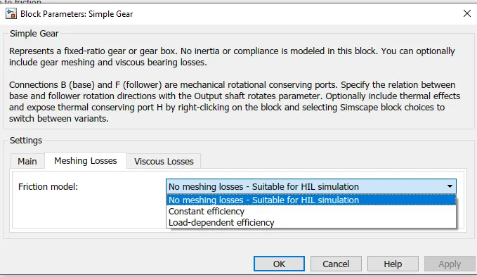
Fig: 2 efficiency cases and no efficiency case

Thermal Model:

You can model the effects of heat flow and temperature change by selecting a thermal block variant. Selecting a thermal variant:

• Exposes port H, a conserving port in the thermal domain.
• Enables the Thermal mass parameter, which allows you to specify the ability of the component to resist changes in temperature.
• Enables the Initial Temperature parameter, which allows you to set the initial temperature.

To select a thermal variant, right-click the block in your model and, from the context menu, select Simscape > Block choices

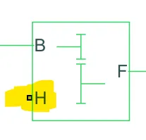
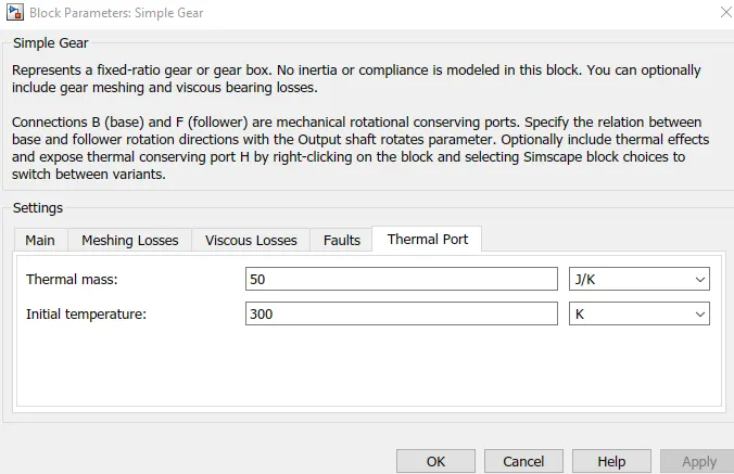
Fig: With thermal port enabled to model thermal effects

Assumptions:

• Gear inertia is assumed negligible.
• Gears are treated as rigid components.
• Coulomb friction slows down simulation. So keep this tradeoff in mind for model fidelity vs runtime

Ports:

• B - Rotational mechanical conserving port associated with the base, or input, shaft.
• F - Rotational mechanical conserving port associated with the follower, or output, shaft.

Parameters:

• Gear ratio - Fixed ratio `g_"FB"` of the follower axis to the base axis. The gear ratio must be strictly positive.
• Motion direction -direction of motion of the follower (output) driveshaft relative to the motion of the base (input) driveshaft.. either in samr or opposite

Friction Models:

Friction models at various precision levels for estimating power losses due to meshing.

• No meshing losses - Suitable for HIL simulation — Neglect friction between gear cogs. Meshing is ideal.
• Constant efficiency — Reduce torque transfer by a constant efficiency factor. This factor falls in the range 0 < η ≤ 1 and is independent from load.
• Load-dependent efficiency — Reduce torque transfer by a variable efficiency factor. This factor falls in the range 0 < η < 1 and varies with the torque load.

Electrical Components/Subsystems:

DC Motor:

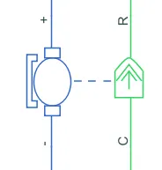
Fig: Simscape Block for Brushless DC motor

Description:The DC Motor block represents the electrical and torque characteristics of a DC motor using the following equivalent circuit model:

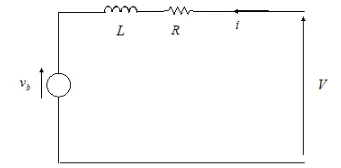
Options for Model parameterization:

• equivalent circuit parameters - which we see above R & L
• rated load and torque
• stall torque and no-load speed

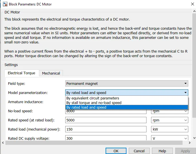
Model paramertixation options

in the other cases the block will convert the given parameters into equivalent circuit parameters and proceed internally.

The DC Motor block assumes that there are no electromagnetic losses. This means that mechanical power is equal to the electrical power dissipated by the back emf in the armature. Equating these two terms gives:

Magnetic field genration:

either permanent magnet or field winding. In case of PM

and in case of field winding

The torque-speed characteristic: for the DC Motor block is related to the parameters in the preceding figure. When you set the Model parameterization parameter to By stall torque & no-load speed or By rated power, rated speed & no-load speed, the block solves for the equivalent circuit parameters as follows:

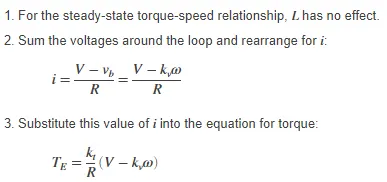
When you set the Model parameterization parameter to By rated power, rated speed & no-load speed, the block uses the rated speed and power to calculate the rated torque. The block uses the rated torque and no-load speed values in the preceding equation to determine values for `R` and `k_t`

After incorporating interia `J` and damping `lambda` the torque eqaution becomes:

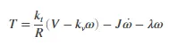
Usually we extimate the rotor damping using the following logic:For no-load, the electrically-generated mechanical torque must equal the rotor damping torque.

`=k_t i_"no-load" = lambda omega_"no-load"`

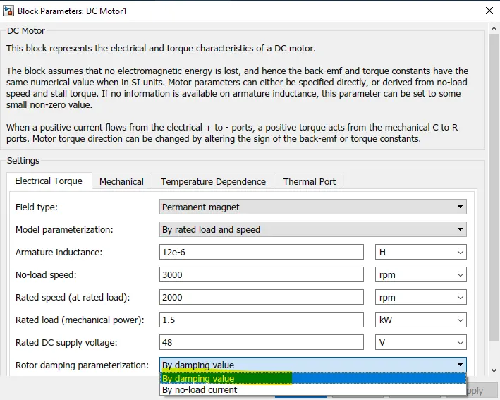
Fig: rotor damping parameterization option

If you select By no-load current for the Rotor damping parameterization parameter, then this equation is used in addition to the torque-speed equation to determine values for λ and the other equation coefficients.

Importance of damping valueThe value for rotor damping, whether specified directly or in terms of no-load current, is taken into account when determining equivalent circuit parameters for Model parameterization options By stall torque and no-load speed and By rated power, rated speed and no-load speed.

When a positive current flows from the electrical + to - ports, a positive torque acts from the mechanical C to R ports.

Ports:

• Positive terminal
• Negative terminal
• C- Motor Case :Mechanical rotational conserving port associated with the DC motor case.
• R- Motor Rotor: Mechanical rotational conserving port associated with the DC motor rotor
• H- thermal port: when thermal model enabled

in case of model parameterization by Rated Load and Speed:

• armature inductance:Inductance of the conducting portion of the motor. If you do not have information about this inductance, set the value of this parameter to a small, nonzero number.
• no load speed:Speed of the motor when not driving a load.
• rated speed: Motor speed at the rated mechanical power level.
• rated load: The mechanical power the motor is designed to deliver at the rated speed.
• DC supply volatge: The voltage at which the motor is rated to operate.

Controlled PWM Voltage:

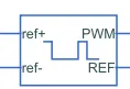
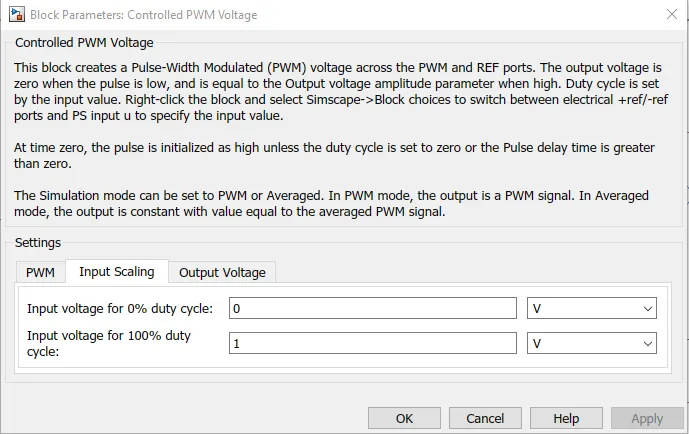
Fig: controlled PWM voltage dialog box

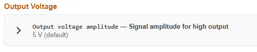
the output is a PWM voltage across the PWM and REF v and will vary between 0 and Output volatge set(i set 2V) for low and high pulse respectively.

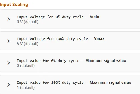
the duty cycle will be decided by the value of the input voltages that are to be given as voltage corresponding to 0% duty cycle and 100% duty cycle respectively.

there are 2 Simulation modes:

• PWM mode - the output will be a PWM signal
• Averaged mode - the output is constant with the value equal to the average of the PWM signal

The block has two modeling variants, accessible by right-clicking the block in your block diagram and then selecting the appropriate option from the context menu, under Simscape > Block choices:

• Electrical input ports — The block calculates the duty cycle based on the reference voltage across its ref+ and ref- ports. This modeling variant is the default. where the demanded duty cycle is calculated as
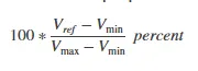
• PS input — Specify the duty cycle value directly by using an input physical signal port.

we have used the electrical input ports where the ref will vary from 0 to 1 that actually comes from the

the value of the output voltage amplitude determines the vlaue of the output voltage.

if we want to use it to drive a motor: given in Documentation

"Do not use the Controlled PWM block to drive a motor block directly. A PWM motor driver goes open circuit in between pulses. Use the H-Bridge block to drive a motor block." as given in the documentation.

and

"When driving a motor via the H-Bridge block, set the Simulation mode parameter to Averaged to speed up simulations. You must also set the Simulation mode parameter of the H-Bridge block to Averaged mode. This applies the average of the demanded PWM voltage to the motor. The Averaged mode assumes that the impedance of the motor inductive term is small at the PWM frequency. To verify this assumption, run the simulation using the PWM mode and compare the results to those obtained from using the Averaged mode."

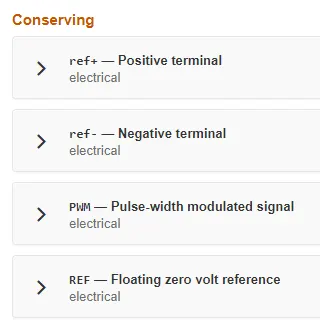
Conserving ports:

Input Scaling

H-Bridge:

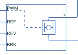
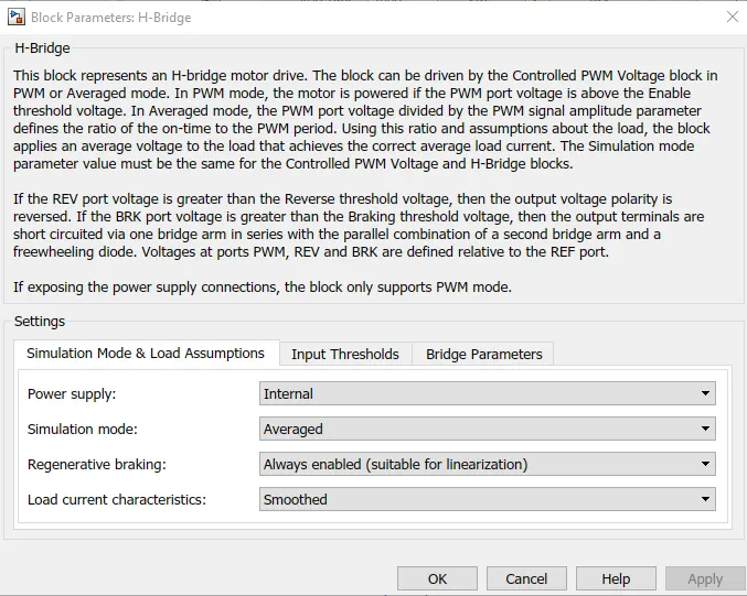
Fig: H-Bridge Dialog Box

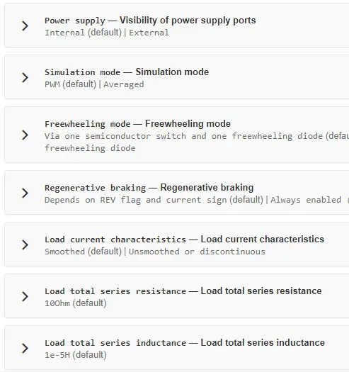
The H-Bridge block represents an H-bridge motor driver. The block has the following two Simulation mode options:PWM & Averaged

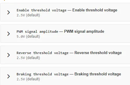
• PWM - The H-Bridge block output is a controlled voltage that depends on the input signal at the PWM port. If the input signal has a value greater than the Enable threshold voltage parameter value, the H-Bridge block output is on and has a value equal to the value of the Output voltage amplitude parameter. If it has a value less than the Enable threshold voltage parameter value, the block maintains the load circuit using one of the three Freewheeling mode options
• Averaged - This mode has two Load current characteristics options:
  • Smoothed
  • Unsmoothed or discontinuous
  • The Smoothed option assumes that the current is practically continuous due to load inductance. In this case, the H-Bridge block output is: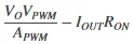

The signal at the REV port determines the polarity of the output. If the value of the signal at the REV port is less than the value of the Reverse threshold voltage parameter, the output has positive polarity; otherwise, it has negative polarity

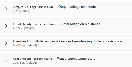
Braking mode is invoked when the voltage presented at the BRK port is larger than the Braking threshold voltage. Regardless of whether in PWM or Averaged mode, when in braking mode the H-bridge is modeled by a series combination of two resistances R1 and R2 where:

• R1 is the resistance of a single bridge arm, that is, half the value of the Total bridge on resistance parameter.
• R2 is the resistance of a single bridge arm in parallel with a diode resistance, that is, R1 · Rd / ( R1 + Rd ), where Rd is the diode resistance.

Conserving ports:

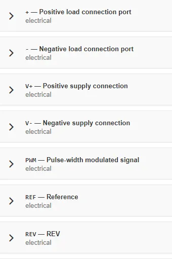
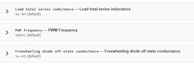
Parameters:

Input thresholds:

Bridge Parameters:

Control Component:

PID controller:

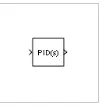
The PID Controller block implements a PID controller (PID, PI, PD, P only, or I only). The block is identical to the Discrete PID Controller block with the Time domain parameter set to Continuous-time.

The block output is a weighted sum of the input signal, the integral of the input signal, and the derivative of the input signal. The weights are the proportional, integral, and derivative gain parameters. A first-order pole filters the derivative action

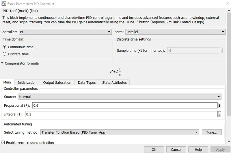
Fig: dialog box of the PID controller block

we see that several controller types and structures.Configurable options include:

• controller type - PID,PI,PD,P only,I only
• controller form - ideal or parallel
• continuous or discrete time
• initial conditons and reset parameters(under initialization tab)
• output saturation limit and anti-windup mechanism(under output saturation tab)
• signal tracking (under initialization tab)
• the last 2 tabs (Data Types and State Attributes) are related to the Fixed-Point designer and State logging for the Code generation purposes for the target hardware and hence no changes are made in them

we can tune the PID gains either manually or using the built in tuner in the Simulink Control Design Software. But we will see that the auto tuner of the built-in PID tuner App will not work because the system is non-linearizable by the app so we will take the approach of Linearizing the plant using the Model Linearizer App and Taking a Simulation Snapshot to get the Offset value for the Plant Identification process.

Where we will Identify a new plant using the system response by getting the I/O data by Simulating the Data. From the simulated response we will try to identify a Plant TF and fit the Plant Simulated data with the identified TF plant data and get the appropriate gains for the system to tune it.

we will see this in the later part. Let us see the model first

Understanding Thermal model and parameters:

for this we can refer to "Simulating Thermal Effects in Rotational and Translational Actuators" in the MATLAB help and understand it better.

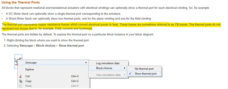
we can see that the thermal port will give out the heat generated by the copper losses of the windings and nothing else so we need to keep this in mind while deifining the Thermal mass and Thermal Circuit to find out the temperature rise.

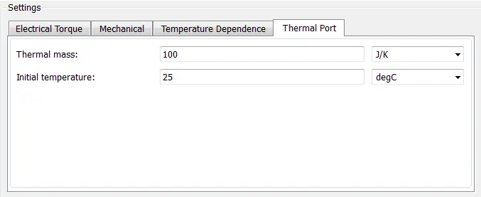
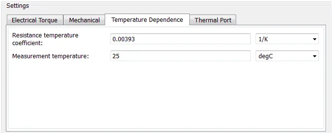
Fig: parmaters enabled to define when Thermal port is enabled in DC motor

Thermal mass: also called Thermal capacitance defines the the energy required to raise the temperature by one degree.

Initial temperature: intital temperature of the component(here motor winding)

Resistance temperature coefficient — Parameter `alpha` in the equation defining resistance as a function of temperature . `=>R = R_0(1 + alpha(T - T_0))`

Measurement temperature — The temperature for which motor parameters are defined.

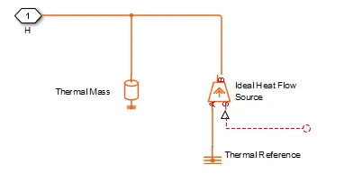
Fig: thermal port model used by the actuator blocks

Explaination:

The heat generated by the copper windings is provided as an input to the S physical signal input port of the Ideal Heat Flow Source. The thermal mass represents the lumped thermal mass of the copper winding where thermal mass is defined as the energy required to raise its temperature by one degree. If the mass is denoted M and the specific heat capacity is cp, then thermal mass is M·cp.

-------------------------------------------------------------------------------------------------------------------

The System Model

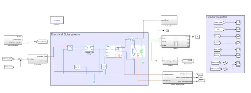
Fig: Complete Model for the System

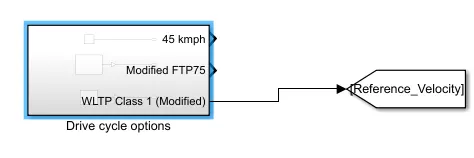
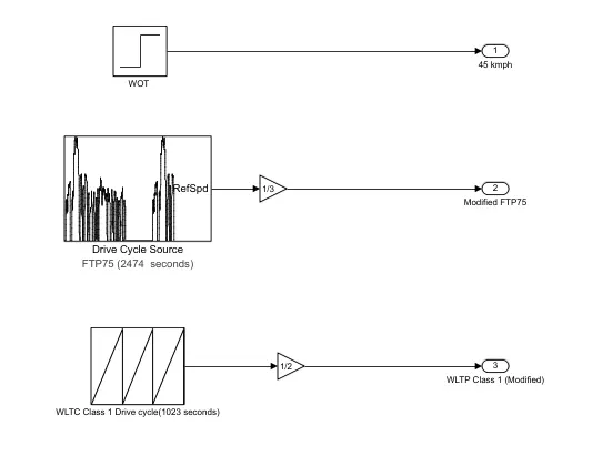
Fig: Drive Cycle Source. Connect required reference Drive cycle for running the model.

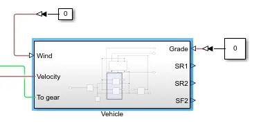
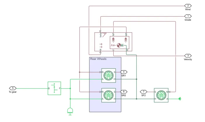
Fig: Vehicle Subsystem - Inside the Vehicle Subsystem Driven by the Motor Mechanical Output

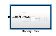
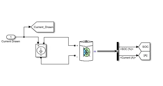
Fig: Battery Pack subsystsem - to find SOC after operation of the vehicle

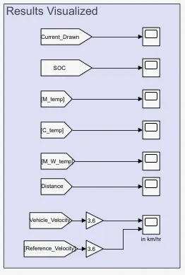
Fig: Simulation Results plotted for different parameters

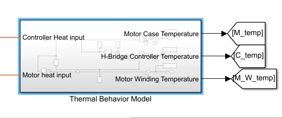
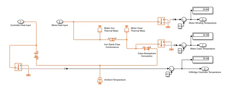
Fig: Thermal behavior subsystem - for the temperature rise in motor and H-Bridge controller

Explaination for the thermal circuit:

we know that the motor has many layers and as we mentioned before the Thermal port of the motor will be only responsible for including the heat generated by the Copper windings. Assuming a motor of weight say 8kg and dimentions 38cm x 28 cm x 16 cm we can get an idea about the amount of the thermal mass for every part of the motor.

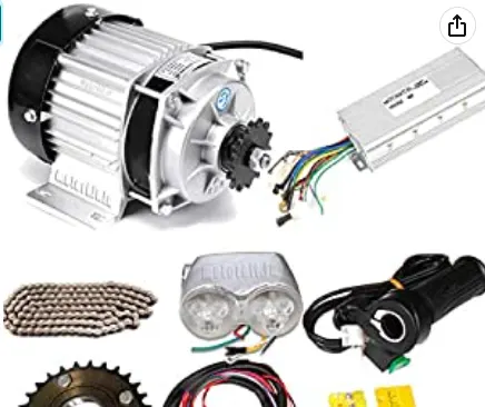
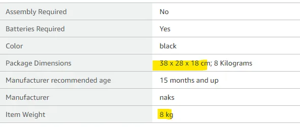
Fig: E-Rickshaw 1kW motor details taken as a reference from Amazon.in (link)

We know that the motor will have several motor layers from which the heat will have to pass in order to reach the outer ambient, these are:

thermal mass as we mentioned was as follows- `"Thermal Mass" = "Specific Heat capacity" xx "Mass"`

• Heat produced from the copper winding. Assuming -1.3 kg copper which is common for a 1kW motor and Specific heat capacity of Copper as 388 J/Kg/K. We will get `=1.3xx388=504.4 J/K` . This is defined in the Motor Parameter itself
• Heat convection to Stator iron case.Assuming -1.2 kg IRON which is common for a 1kW motor and Specific heat capacity of Copper as 447 J/Kg/K.
• Heat conduction from the iron stator stack to the motor case.
  • for the conduction : Keeping the Dimentions of our reference motor we can say the area of contact is `=2xxpixx(38/2 -2)xx28 = 3166.73 cm^2`, thickness to be `3 cm` and thermal condictivity of `80 W/(m*K)`
  • for the motor case : 1.5 kg casing which is common for a 1kW motor and Specific heat capacity of Case material as 903 J/Kg/K.
• Case to the ambient Convection . Area `=2xxpixx(38/2)xx28 = 3342.73 cm^2` and a typical air heat transfer coefiicient of `50 W/(m^2 K)`

for the H-Bridge controller:

• only controller to ambiance convection is considered and Area fo the controller board is considere to be `=10 cm^2 =0.01 m^2 ` and a typical air heat transfer coefiicient of `50 W/(m^2 K)`but we increase it to `130 W/(m^2 K)` considering certain passive cooling like heat sinks. and a little forced convection. This is because since the area is very small for heat exchnage the air velocity and air temperature is very important.

where the different parameters can be seen from the following site and the corresponding heat transfer coeffienct can also be calculated automatically, fo example, based on my inputs like 8 m/s `u_m` which is air velocity the following was the value

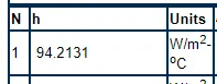
other thermal circuit parameters and construction is from MATLAB documentation(reference and reference2)

Note: it is assumed the E-Rickshaw starts from rest so the Ambient Temperature and Initial temperature of all Subsystems is same and is assumer to be 298.15 K

the System Blocks:

• Some reference to track - Speed VS time - A drive cycle
• Conveter to convert Linear Parameters to Electrical parameters - acceleration and deceleration commands from PI controller and controlled voltage source. to create the relevant Acceleration and Decelleration commands
• Controlled electrical signals - created by the Controlled PWM Voltage
• Motor Driver - H-bridge motor drive that will use the electrical signals corresponding to acceleration and deceleration into appropriate voltage for the motor to be driven in terms of magnitude and polarity
• Motor - the motor used to convert the elctrical signals/energy into mechanical output required to obtain the desired speed vs time performance
• Mechanical gear - to couple/link the motor shaft with the vehicle transmission
• Wheels - to apply the angular motion that it receives from the gear to the wheels and get the correspoding response from the vehicle body and driving condtions
• vehicle body - to model the vehicle parameters as well as the road conditions and get the velocity output that will be compared with the desired output to assess the performance of the model
• current measurement and integration - to get the total amount of discharge done in order to determine the state of charge using the coulomb counting method
• battery - to provide the electrical energy for the system to run

System level configuration & model Parameters:

the vehicle body chosen is as follows:

• Mass: `400 kg`
• Wheels per axle: `2` . with one wheel on the forward side.
• Frontal area : `1.6 m^2`
• wheel radius: `0.37 m`

external conditions chosen :

• Air density:`1.18 (kg)/(m^3)`
• Drag coefficient : `0.55`

motor:

• no load speed: `3000 "rpm"`
• rated speed: `2000 "rpm"`
• rated load: `1kW`
• rated DC Supply:`48V`

H-Bridge:

• Output voltage aplitude:`48V`
• enable threshold voltage: `0.1V`
• PWM signal amplitude: `2V`

Controlled PWM Voltage:

• Output voltage: `2V`
• Input scaling: `0 to 1`
• frequency: `1000Hz`

Drive cycle used: FTP75 (2474s) scaled by `1/3`

As we mentioned earlier the goverment rgulation on top speed as well as evident in the market products we do not need Drive cycle with speeds higher than 25kmph so we divided the FTP75 by 3 for a drive cycle with top speed as 30.38 kmph

therefore the DC Motor parameters can be set as:

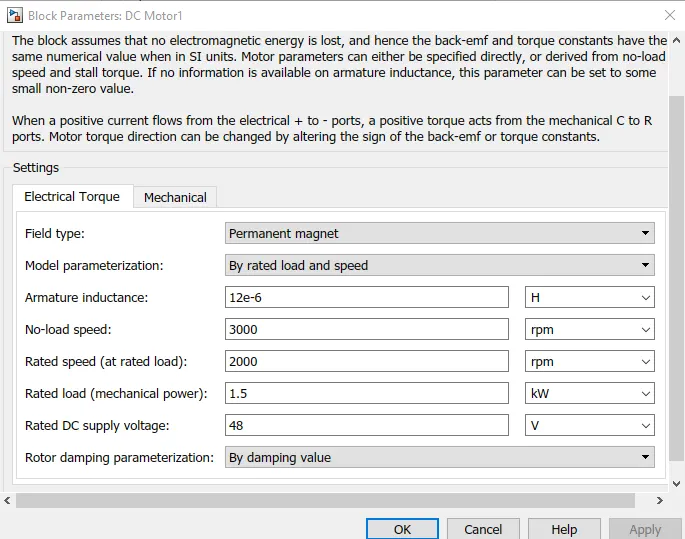
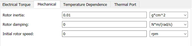
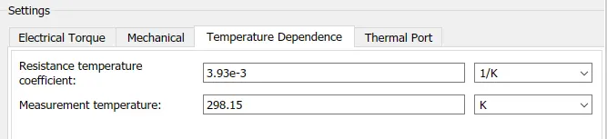
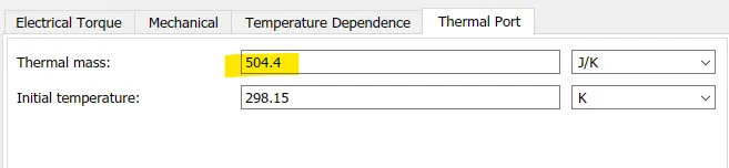
DC motor parameters

since the DC Supply Voltage is 48V then the Motor Driver H-Bridge should also have Output voltage as 48V

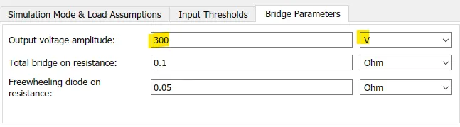
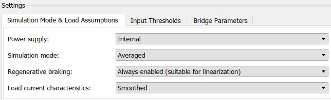
and power supply is kept internal as in case of external we have only the PWM Simulation mode avaialable and that would take the simulation to run in a lot of time.

regenerative braking is always enabled as that is how actually our controller operates to ensure regenerative braking. and Load characterstics are Smoothed as it is assumed continuous due to practical load inductance.

controlled PWM voltage should give us the same voltage that is in the input threshold of the Hbridge in the PWM signal parameters

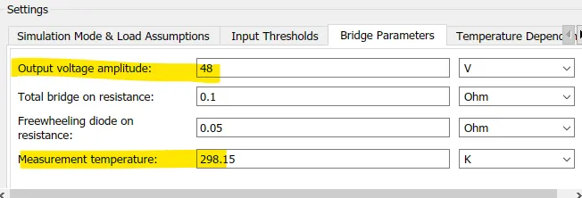
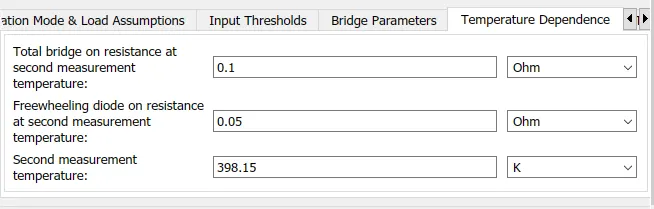
which is 2 V here so for the Controlled PWM voltage the output should also be 5V as w can see

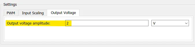
now for running the PWM controlled voltage we need to understand the range of the signal for scaling the 0% to 100% PWM signal. Since the input signal is coming from the PI contoller which gives us the Acceleration and Decceleration commands clubbed together. We have chosen the Input scaling to be 0 to 1 for the Controlled PWM voltage that will drive the H-Bridge forward movement then we should limit the output from the controller to 1

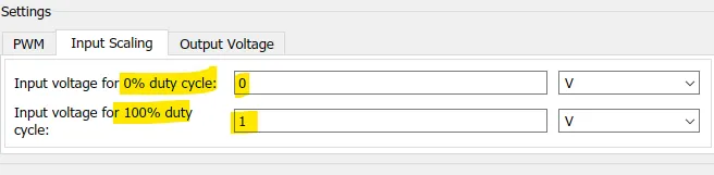
we need to seperate the commands for Acceleration and braking and also limit the Forward/Acceleration input from 0 to 1 in order to match the Controlled PWM Input scaling:

for this we need to seperate the signals according to the sign of the output signal from the PID contoller and feed the positive part to the controlled PWM to feed the PWM of H-bridge and the negative to feed the BRK brake nput of the H-Bridge block. The arrangement is shown below.

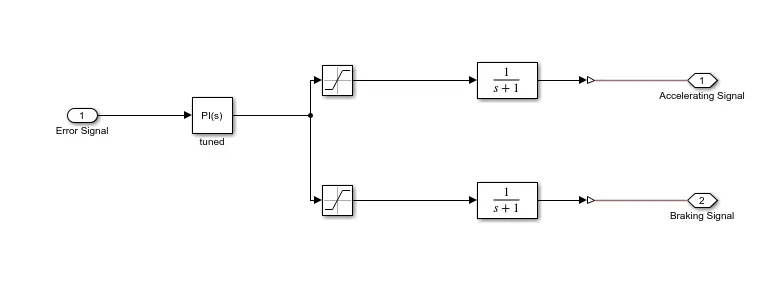
Fig: Arrangement to show the splitting of the PID control signal into positive and negative scaled saturated iputs for the H-Bridge and Controlled PWM

Note:use of Transfer Function block is done as a Filter . This is to avoid the Algebraic loop error beacuse saturation computation is a computation that does not take time or cause delay that may cause error in the model . so we can either use a filter as above or a delay to avoid the algebraic error.

Saturation limits is required in Positive part from 0 to 1 to match the Controlled PWM input scaling(we can also put the upper limit as +inf the Controlled PWM will respond the same to signal value hogher than 1 as 1 i.e. 100%) and in Negative part it can be from 0 to -inf or -1 since it is directly fed to the H-Bridge. Important part is that the Posotive and Negative part of the signal is fed to the appropriate blocks.

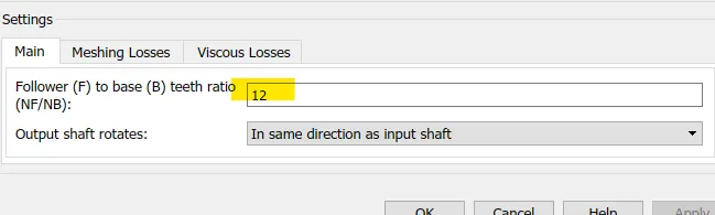
for the Gear ratio an appropriate ratio of 6 is chosen taking into consideration the wheel radius an the Motor RPM

for estimation of charge we have chosen to assume a battery pack made of Cells with Nominal Voltage 3.7V and Nominal Capacity 3.6Ah

from the simualtion we will see the current drawn from the motor reaches upto 300A

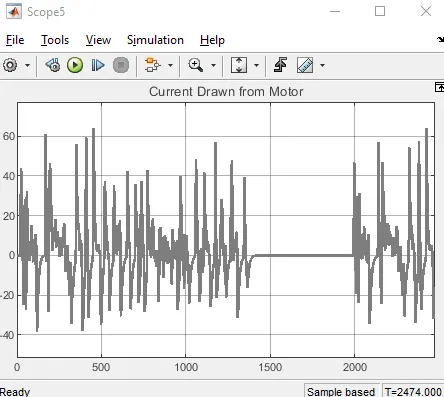
assuming the battery to be able to sustain 2.5C discharge rate easily we can say that the capacity of the battery will be 60/2.5 = 24Ah which means 240/3.6=6.67 = 7 cells in parallel

and for the no of cells in series we know the motor voltage rating is 48V = 48/3.7 = 12.97= 13 cells in series . So the pack will be 13S7P

So the Battery Capacity is :

`=3.7V xx 3.6Ah xx 13 xx7 = 1212.12 Wh = 1.21 kWh`

this will be implemented as the battery with the above conguration and nominal ratings as:

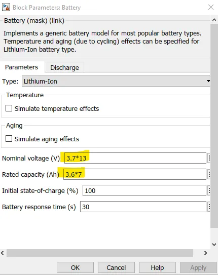
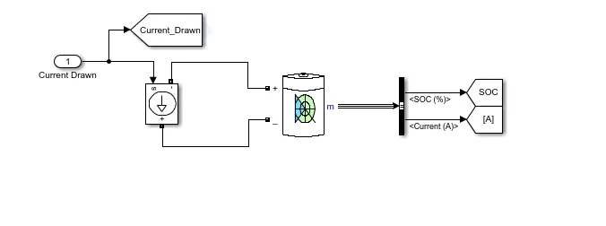
Fig: 3.7V and 3.6Ah in 13S7P configuration and Battery Arrangment. Current drawn from the Controlled current source being fed by the Motor Current sensed

so after running the simulation we will see the depletion in the soc after 2474s running on the modified FTP75 drive cycle.

Findind the PI Gains:

after trying to tune the PI gains using the auto tuner we will find that the model cannot be linearized this is because it is inherently Non-Linear in nature and MATLAB tuner failed to linearize the model to create a LTI Small Signal Model.

So we will have to use the Simulated Data to Identify the Plant and then use that behavior information from the simulated data to find the PI gains for the model.

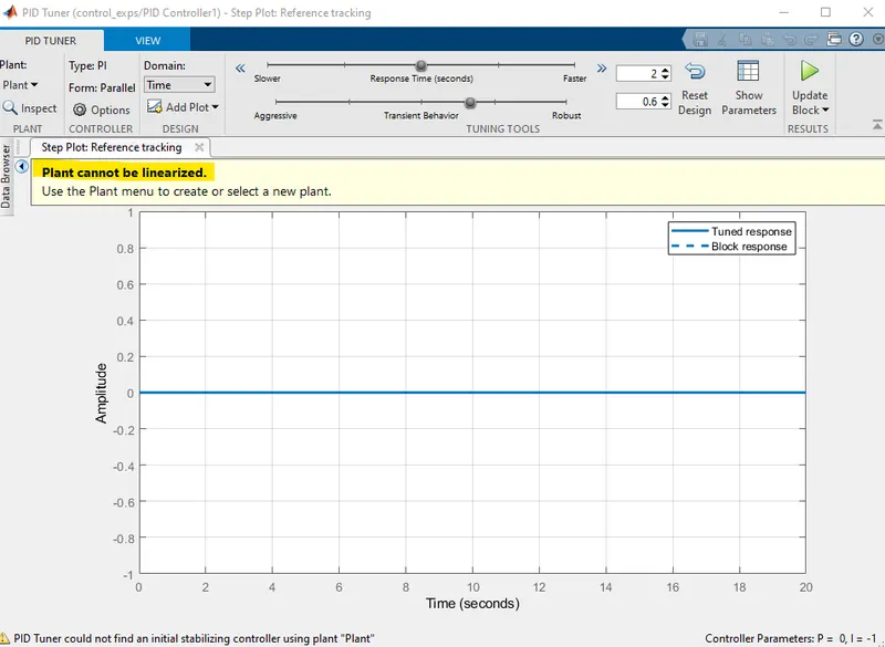
Fig: PLant not linearized by auto-tuner Simulink

now open the PID tuner and use the Identify New Plant and then I/O data> Simulate Data

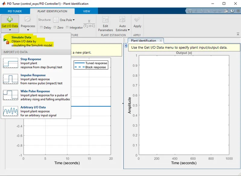
Fig: Plant Identifcation Using Simulated Data

Use the Step Input with the same parameters as in the model and Simulate the plant

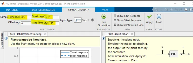
Fig: Plant identification Step Signal same as the step applied in Model Linearizer

Run the Simulation

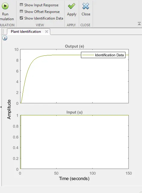
Fig: Simulated Data For Plant Identification

click Apply and close

Run the Plant Identification

now adjust the Simulated Data and the Identifed Plant data so they over lap closely

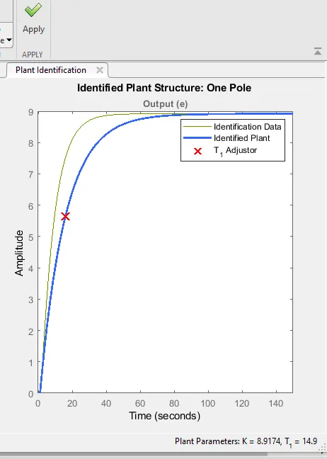
Fig: Adjust the Identified Plant and so it matche Simulated data closely and click Apply

plant response with new gains from the simulated data:

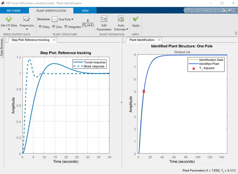
Fig: Plant data Tuned VS before

Now close the PLant idenfication tab and tune the response for desired behavior using the sliders and apply

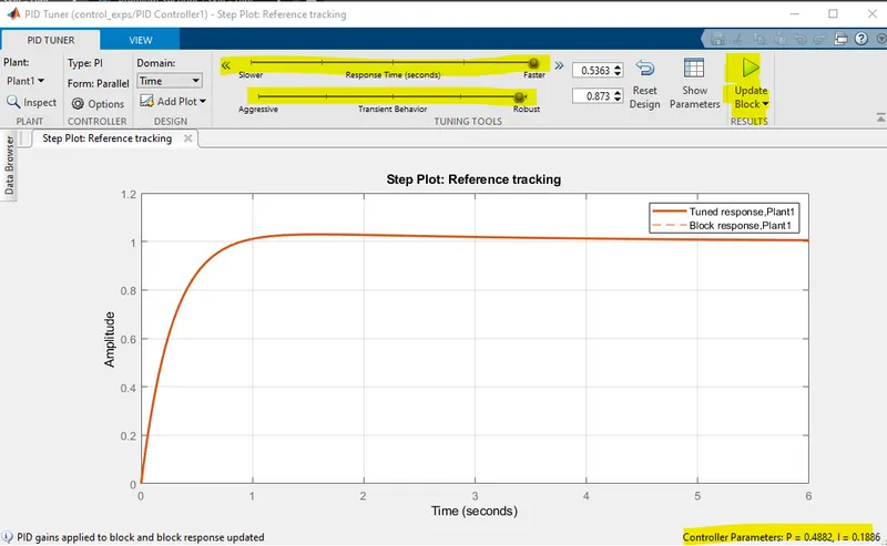
Fig: behavior after tuning using the Slider. And Update the Block. See the updated gains at the bottom

i settled on the Gain Values of : `K_p = 0.7` and `K_i = 0.07`

Running the Simulation: Results

Drive Cycle : Modified FTP75

Simulation time: 2474s and `K_p = 0.7` and `K_i = 0.07`

after running the simulation for 2474s we will observe the results

Distance

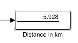
total distance travelled by the vehicle in 2474s of the modified FTP75 Drive cycle

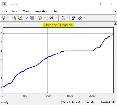
Distance VS time

Reference(Drive Cycle) Tracking

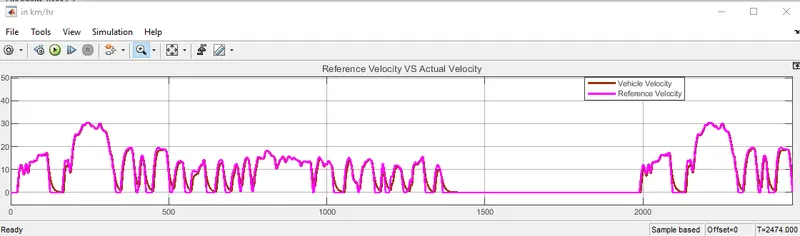
Fig: FTP75 input Drive cycle (majenta) and actual response of the vehicle(brown) with `K_p = 0.7` and `K_i = 0.07`

Observation: we see that the response of the vehicle matches the required response closely and changes are captured in a timely manner.

State of Charge Depletion and Range

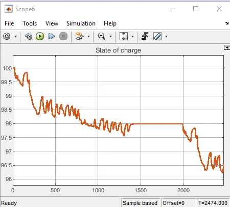
Fig: State of charge. Depletion of charge from 100% to 96.56% . Total Deplection go 3.44% in 2474s

so from this we can also find the range of the vehicle for modified FTP75 drive cycle. Since we saw for one complete FTP75 cycle the distance covered was `5.928 km` and charge depletion was `3.44 %` so for DoD of say `90%` the total number of modified FTP75 cycles will be `=90/3.44 = 26.163 "cycles"`

as for 1 cycle the distance covered was 5.928 km the range should be `=26.163xx5.928 = 155.094 km`So Range will be 155.094 km .Which is very similar to the market available products we saw of around 120Km , it is a bit larger (155Km) but in real life it will end up smaller since many physical phenomenon were left unmodellled such as Brake friction loss,uneven road surface,variation in payload/passengers etc.

Current Drawn

Fig:Current Drawn from the motor corresponding to the modified FTP75 drive cycle

Thermal Behavior

Motor Temperature(Casing): degC

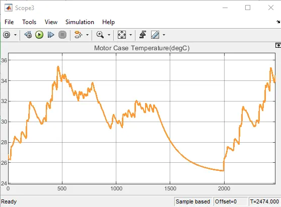
Fig: Rise in Motor Temperature. We see it reaches upto 35.4 deg Celcius

Motor Temperature(Winding):degC

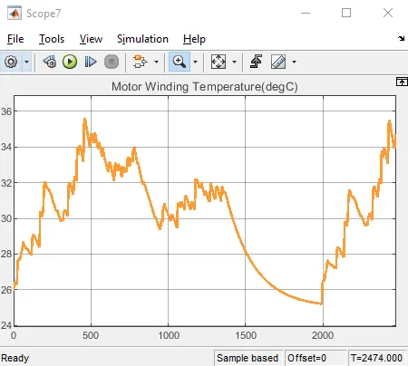
Fig: Rise in Motor Winding Temperature. We see it reaches upto 35.60 deg Celcius

Controller Temperature:deC

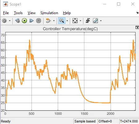
Fig: H-Bridge conveter temperature. We see that it rises upto 66.8 deg Celcius

this means we need to increase the cooling of it through more forced air or even liquid cooling can be considered.

Drive Cycle : Modified WLTP(Worldwide Harmonized Light Vehicles Test Procedure) Class 1

Simulation time: 1023s and `K_p = 0.7` and `K_i = 0.07`

after running the simulation for 1023s we will observe the results

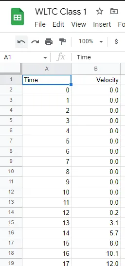
Fig: WLTP class 1 .xlxs file

Distance

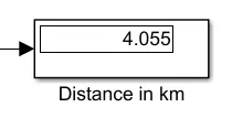
total distance travelled by the vehicle in 1023s of the modified WLTP Class 1 Drive cycle

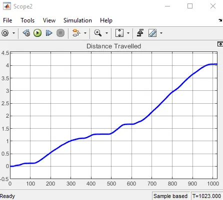
Distance VS time

Reference(Drive Cycle) Tracking

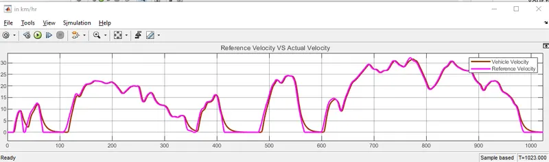
Fig: Modified WLTP Class 1 input Drive cycle (majenta) and actual response of the vehicle(brown) with `K_p = 0.7` and `K_i = 0.07`

Observation: we see that the response of the vehicle matches the required response closely and changes are captured in a timely manner.

State of Charge Depletion and Range

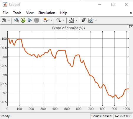
Fig: State of charge. Depletion of charge from 100% to 97.23% . Total Deplection go 2.77% in 1023s

so from this we can also find the range of the vehicle for modified WLTP Class 1 drive cycle. Since we saw for one complete WLTP Class 1 cycle the distance covered was `4.055 km` and charge depletion was `2.77 %` so for DoD of say `90%` the total number of modified WLTP Class 1 cycles will be `=90/2.77 = 32.49 "cycles"`

as for 1 cycle the distance covered was 4.055 km the range should be `=32.49xx4.055 = 131.75 km`So Range will be 131.75 km .Which is very similar to the market available products we saw of around 120Km , it is a bit larger (155Km) but in real life it will end up smaller since many physical phenomenon were left unmodellled such as Brake friction loss,uneven road surface,variation in payload/passengers etc.

Current Drawn

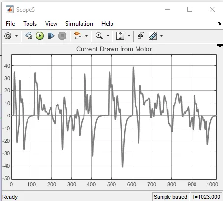
Fig:Current Drawn from the motor corresponding to the modified WLTP Class 1 drive cycle

Thermal Behavior

Motor Temperature(Casing): degC

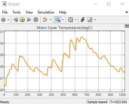
Fig: Rise in Motor Temperature. We see it reaches upto 30.56 deg Celcius

Motor Temperature(Winding):degC

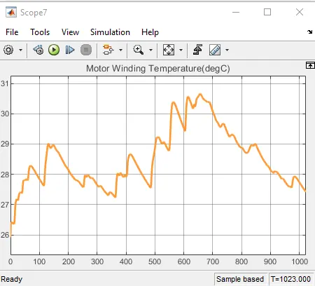
Fig: Rise in Motor Winding Temperature. We see it reaches upto 30.66 deg Celcius

Controller Temperature:deC

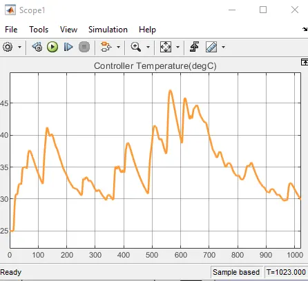
Fig: H-Bridge conveter temperature. We see that it rises upto 47.05 deg Celcius

Drive Cycle : WOT 45kmph

Simulation time:150s and `K_p = 0.7` and `K_i = 0.07`

Now coming to the 45 kmph: Since mentioned earlier this model was based on Market available products and there is a government regulation for the top speed of 25kmphr

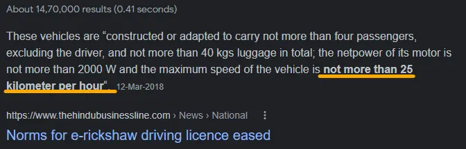
Fig: first google result of the "E-rickshaw top speed Government regulation" search

the following E-ricshaw was designed for that.

Running the Simulation for 45 kmphr let us inspect the result.

Reference(Drive Cycle) Tracking

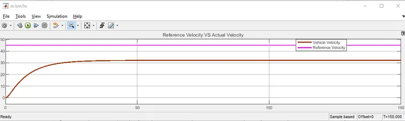
Fig: WOT 45kmph input (majenta) and actual response of the vehicle(brown) with `K_p = 0.7` and `K_i = 0.07`

Observation: as we can see that since the E-Rickshaw had specific parameters it has a limited top speed of 32.13 kmph which after including the non captured dyanamics will lead to somewhat close to the 25kmph regulated speed.

Current Drawn

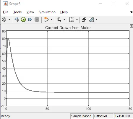
Fig:Current Drawn from the motor corresponding to the WOT drive cycle

Thermal Behavior

Motor Temperature(Casing): degC

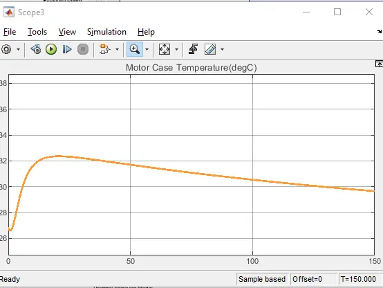
Fig: Rise in Motor Casing Temperature. We see it reaches upto 32.35 deg Celcius

Motor Temperature(Winding):degC

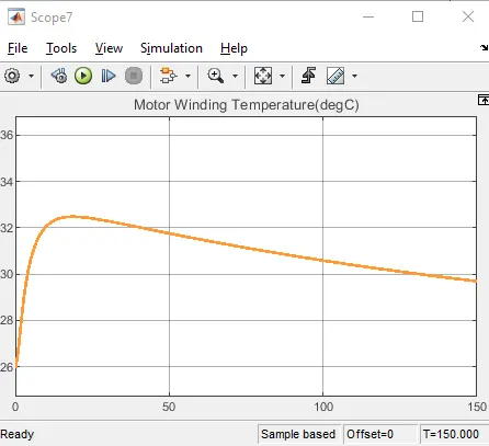
Fig: Rise in Motor Winding Temperature. We see it reaches upto 32.45 deg Celcius

Controller Temperature:deC

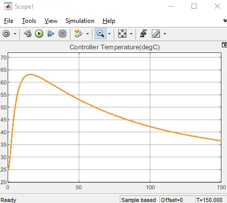
Fig: H-Bridge conveter temperature. We see that it rises upto 66.8 deg Celcius

this means we need to increase the cooling of it through more forced air or even liquid cooling can be considered.

we can also run the simulation a bit longer to find out the Thermal Equilibrium at aroung 900 s

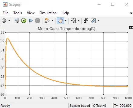
Fig: depicting thermal equilibrium reached by motor after around 900 s of WOT applied

So we need to make some changes so that we can achive the 45kmph speed required for part 2 :

this can be done in multiple ways or a combination of them ,some of them can be:

• Decreasing payload mass(limited to kerb weight of 190kg)
• Increasing motor size and RPM

After trying to match the result using the above two approches we settle onto the following:

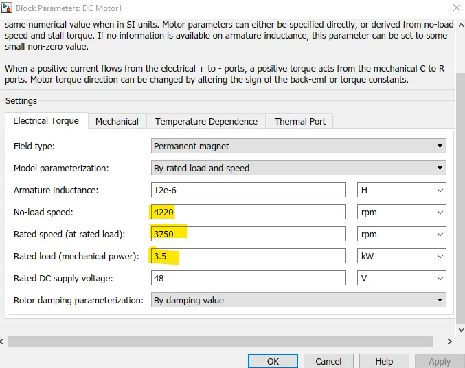
Fig: new motor rating and specification that will give us the required top speed

New motor has:

• No load speed:4220 RPM
• Nominal/Rated Speed:3750 RPM
• Rated Power: 3.5 kW

the Vehicle load has also been reduced to only its kerb weight : 190kg

Reference(Drive Cycle) Tracking

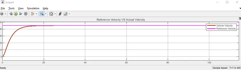
Fig: WOT 45kmph input (majenta) and actual response of the vehicle(brown) with `K_p = 0.7` and `K_i = 0.07`

Observation: as we can see that since the E-Rickshaw with the new parameters it has a top speed of 45 kmph

Current Drawn

Fig:Current Drawn from the motor corresponding to the WOT drive cycle

Thermal Behavior

Motor Temperature(Casing): degC

Fig: Rise in Motor Casing Temperature. We see it reaches upto 32.35 deg Celcius

Motor Temperature(Winding):degC

Fig: Rise in Motor Winding Temperature. We see it reaches upto 32.45 deg Celcius

Controller Temperature:deC

Fig: H-Bridge conveter temperature. We see that it rises upto 66.8 deg Celcius

For 100 km constant speed driving at 45kmph: energy consumption,motor and controller temperature ,etc are as below

the model will remain the same and we just have to terminate the simulation when we have travelled a distance of 100km. This is realized as below:

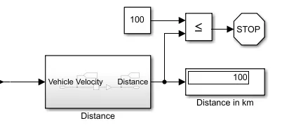
Fig: implementation of the 100km criteria. Simulation will stop when 100 km is reached

So for the E-Rickshaw to cover 100km the time required will be:

`=>"Time" = "Distance"/"Speed" = (100 km)/(45 (km)/(hr))=2.2222 hr = 8000 sec`

which is very close to the simulation result:

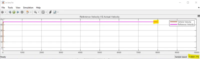
Fig: Simulation terminated near 8000s (8001.77s)

Why not exact 8000s? this is because in the beginning the Richshaw takes time to accelerate from 0kmph to 45kmph and that additional time is added .

Distance

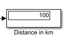
total distance travelled by the vehicle in 2474s of the modified FTP75 Drive cycle

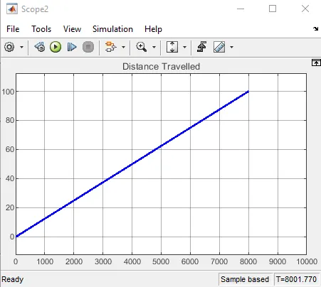
Distance VS time

Reference(Drive Cycle) Tracking

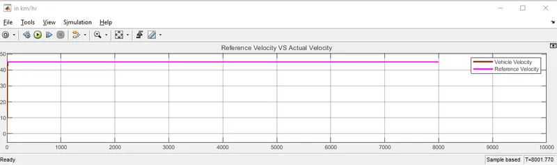
Fig: 45kmph WOT input (majenta) and actual response of the vehicle(brown) with `K_p = 0.7` and `K_i = 0.07`

State of Charge Depletion and Range

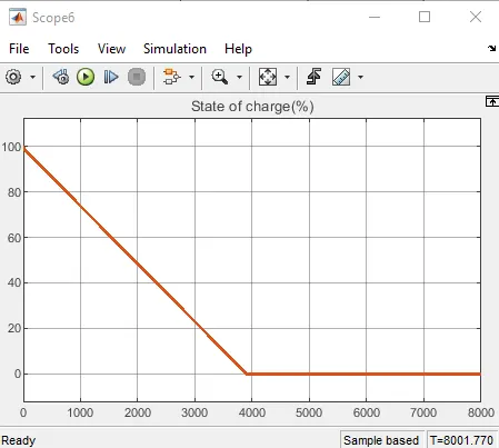
Fig: State of charge. Depletion of charge from 100% to 0% in t=3902.34s.

so from this we can also find the range of the vehicle for 45kmh WOT drive cycle and the new Motor configuration is much less than 100 km. So we can find out the range by zooming in , SOC becomes ) at t=3902.34s and the corresponding distance travelled here is 48.74 Km.

Current Drawn

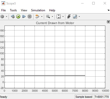
Fig:Current Drawn from the motor corresponding to the modified FTP75 drive cycle

Thermal Behavior

Motor Temperature(Casing): degC

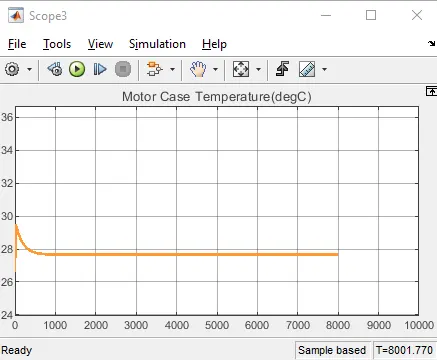
Fig: Rise in Motor Temperature. We see it reaches to equilibirum temperature 27.65 deg Celcius around t=1850s

Motor Temperature(Winding): degC

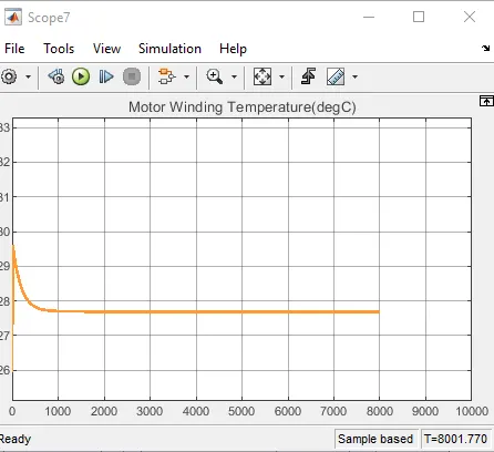
Fig: Rise in Motor Winding Temperature. We see it reaches to equilibirum temperature 27.69 deg Celcius around t=1900s

Controller Temperature:deC

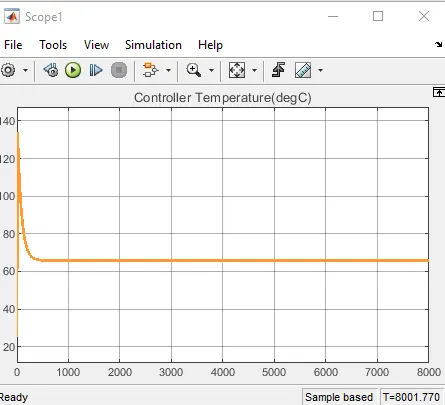
Fig: H-Bridge conveter temperature. We see it reaches to equilibirum temperature 65.84 deg Celcius around t=850s

this means we need to increase the cooling of it through more forced air or even liquid cooling can be considered.

Energy Consumption: Since we see it depleted the 13S7P Battery pack of 3.7V 3.6Ah cells

`=3.7V xx 3.6Ah xx 13 xx7 = 1212.12 Wh = 1.21 kWh`

in only 3902.4s that and it further goes upto 8001.8 seconds we can roughly calculate the Energy consumed as.

1212.12 Wh consumed in 3902.4 sec ,

`=8001.8/3902.4 xx "total capacity"= 2.051 xx 1.21 kWh = 2.485 kWh`

So total enrgy consumed is 2.485 kWh.

Sheet with Assumed parameters is also added:

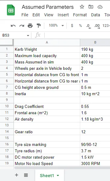
Fig: Assumed parameters img(attatched)