Final Project: Electric Rickshaw modelling

AIM:Create a detailed MATLAB model of an electric rickshaw (three wheel passenger vehicle) as per details.

OBJECTIVE:

1)Rear wheels driven by PM brushed type motor

2)Assume efficiency points of motor controller and motor

3)Make an excel sheet of all input and assumed data

4)Results: For any three standard driving cycles show energy consumption, temperature rise of motor and controller for 100 km constant speed driving at 45 kmph.

INTRODUCTION:

Electric Rickshaw: They are being widely accepted as an alternative to petrol/diesel/CNG auto rickshaws. ... They are three-wheelers powered by an electric motor ranging from 650 to 1400 Watts. They are mostly manufactured in India and China, only a few other countries manufacture these vehicles.

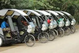
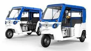
Electric rickshaws (also known as electric tuk-tuks or e-rickshaws or toto or e-tricycles) have been becoming more popular in some cities since 2008 as an alternative to auto rickshaws and pulled rickshaws because of their low fuel cost, and less human effort compared to pulled rickshaws. They are being widely accepted as an alternative to petrol/diesel/CNG auto rickshaws. They are three-wheelers powered by an electric motor ranging from 650 to 1400 Watts. They are mostly manufactured in India and China, only a few other countries manufacture these vehicles. Battery-run rickshaws could be a low-emitter complementary transport for the low-income people, who suffer most from a lack of transport facility, if introduced in a systematic manner according to experts.

Design and construction

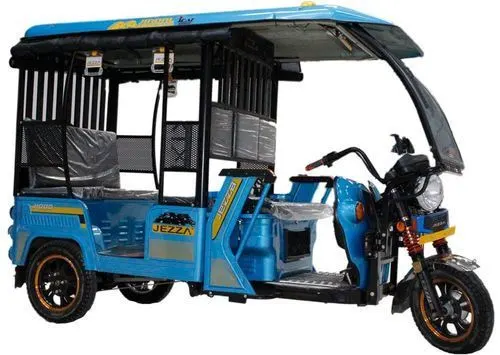
These rickshaws have a M.S(Mild Steel) tubular Chassis, consisting of three wheels with a differential mechanism at the rear wheels. The motor is brushless DC motor manufactured mostly in India and China. The electrical system used in Indian version is 48V and Bangladesh is 60V. The body design from most popular Chinese version is of very thin iron or aluminum sheets. Vehicles made in fiber are also popular because of their strength and durability, resulting in low maintenance, especially in India. Body design is varied from load carriers, passenger vehicles with no roof, to full body with windshield for drivers comfort.It consist of a controller unit.They are sold on the basis of voltage supplied and current output, also the number of mosfet(metal oxide field effect transistors) used. The battery used is mostly lead acid batteries with life of 6–12 months. Deep cycle batteries designed for electric vehicles are rarely used. Weight of the electric car has also been a recurring design difficulty in them.

Below is an Erickshaw 3 wheeler model using Lithium ion battery with the following Technical specifications

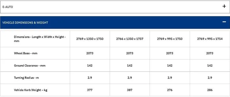
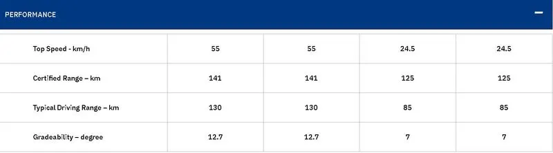
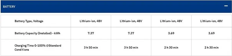
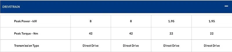
We have Designed a similar kind of a model with Lithium ion battery using MATLAB simulink blocks and simulate the model with 3 different drive cycles.

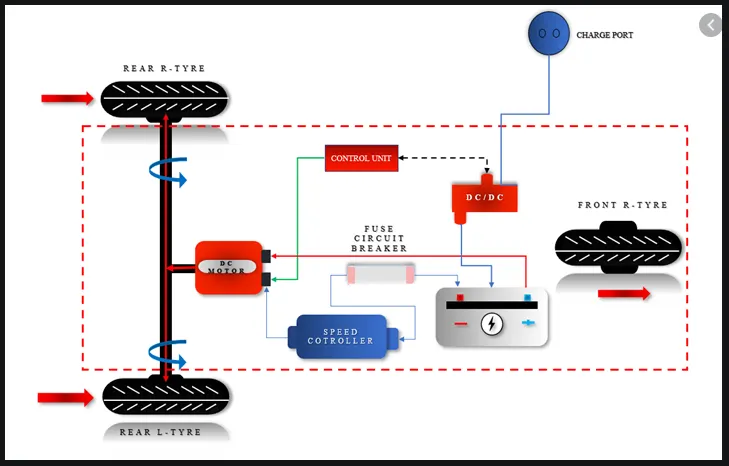
Drive Train Image of Electric Erickshaw

Procedure:

An electric autorickshaw should have the following components to simulate in virtual environment:

1. Electric motor and Gear system
2. Power Controller
3. Vehicle dynamics
4. Battery
5. Driver configuration
6. Drive cycles

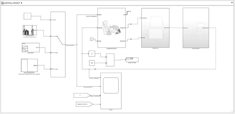
All of these components are represented in different subsystems in the model. We will discuss all these blocks as per their functions and how they work. When all the subsystems are arranged together as a model for electric rickshaw, this how the model looks.

MATLAB Model of Electric Rickshaw

Design and Specifications of Model Components and its Parameters:

1)ELECTRIC PLANT[MOTOR & CONTROLLER] SUB SYSTEM:

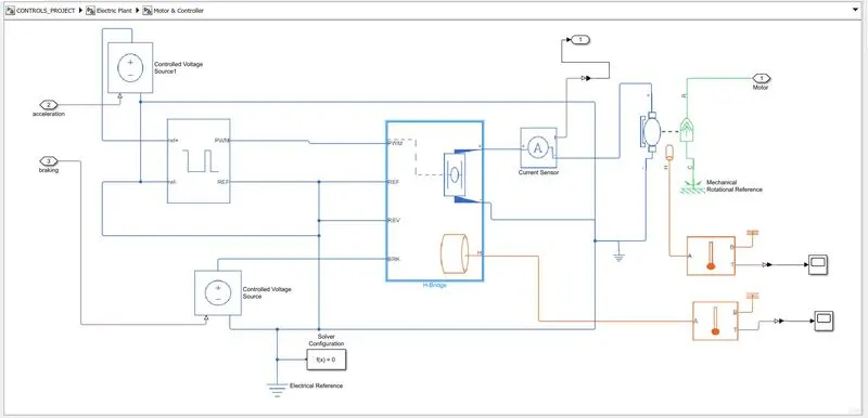
The components,blocks and block parameters involved in this subsystem are discussed below

Electric motor and Gear system:

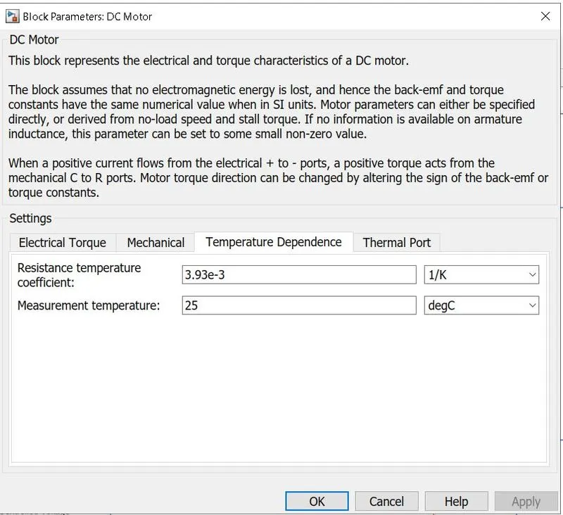
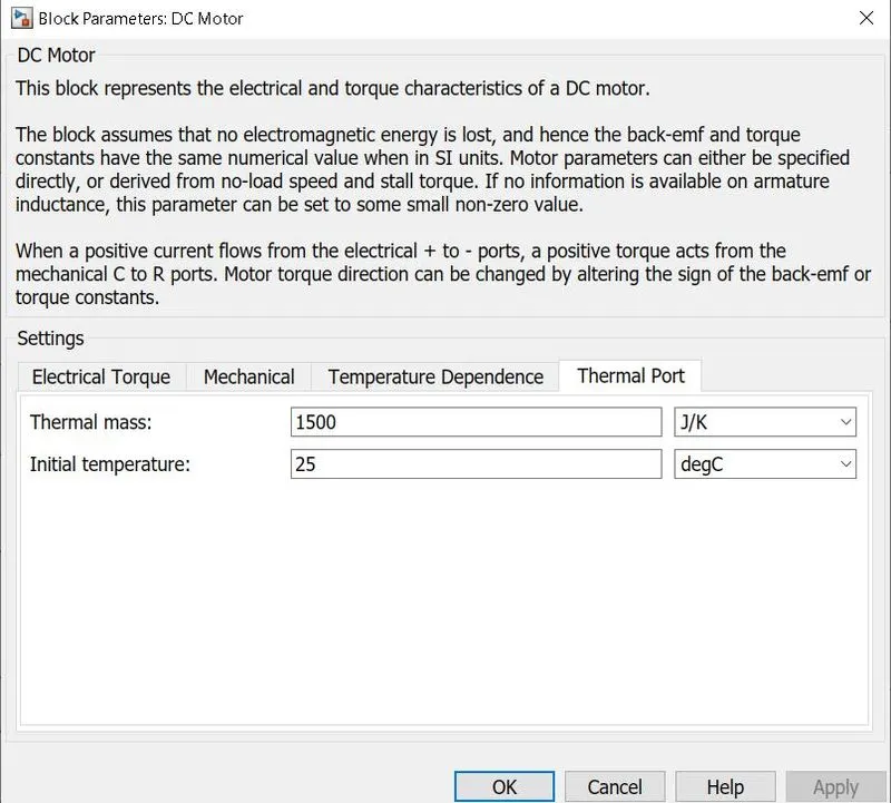
This subsystem uses a DC motor block with thermal port to get the temperature of the motor. The motor is connected to electrical terminals coming out of the power controller. The motor specifications are set properly and motor type is set to Permanent magnet type. This block has mechanical part as well, one end of which is connected to the mechanical rotational reference and other to the gear box. The gear box has a gear ratio of 5. There is a gear output taken from this subsystem and given to the vehicle dynamics system.

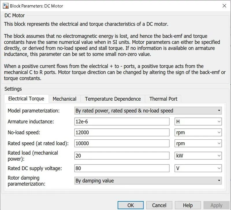
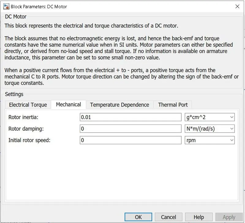
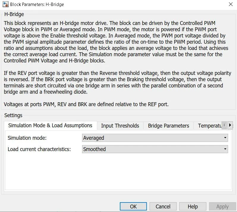
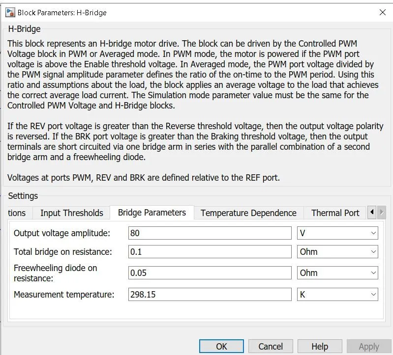
2)Power Controller: This subsytem is of prime importamce in electric powertrains. The controller does the main work of limiting and providing the required voltage. The system uses an H-Bridge block, controlled PWM voltage block, two controlled voltage source blocks for acceleration and deceleration(braking). This is because the system has regenrative braking. The H-bridge calculates the current drawn from the battery for the generated PWM voltage. This current is given to the motor. This current is also sensed and the same is removed from and supplied to the battery. The H-bridge also has a thermal port and it is connected to the temperature sensor to know the controller temperature.

H-Bridge:

This block represents an H-bridge motor drive. The block can be driven by the Controlled PWM Voltage block in PWM or Averaged mode. In PWM mode, the motor is powered if the PWM port voltage is above the Enable threshold voltage. In Averaged mode, the PWM port voltage divided by the PWM signal amplitude parameter defines the ratio of the on-time to the PWM period.Using this ratio and assumptions about the load, the block applies an average voltage to the load that achieves the correct average load current. The Simulation mode parameter value must be the same for the Controlled PWM Voltage and H-Bridge blocks.

If the REV port voltage is greater than the Reverse threshold voltage, then the output voltage polarity is reversed. If the BRK port voltage is greater than the Braking threshold voltage, then the output terminals are short circuited via one bridge arm in series with the parallel combination of a second bridge arm and a freewheeling diode. Voltages at ports PWM, REV and BRK are defined relative to the REF port.

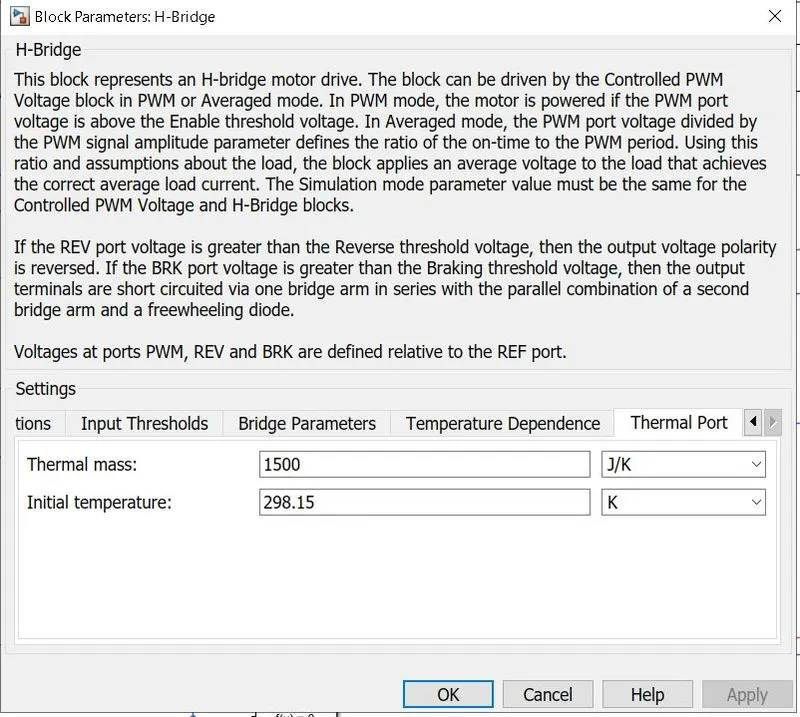
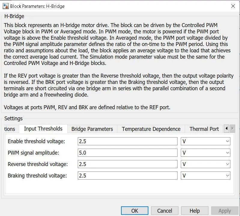
Temperature Sensor:

This block measures temperature in a thermal network. There is no heat flow through the sensor. The physical signal port T reports the temperature difference across the sensor. The measurement is positive when the temperature at port A is greater than the temperature at port B.

Controlled PWM Voltage:

This block creates a Pulse-Width Modulated (PWM) voltage across the PWM and REF ports. The output voltage is zero when the pulse is low, and is equal to the Output voltage amplitude parameter when high. Duty cycle is set by the input value. Right-click the block and select Simscape->Block choices to switch between electrical +ref/-ref ports and PS input u to specify the input value.

At time zero, the pulse is initialized as high unless the duty cycle is set to zero or the Pulse delay time is greater than zero.

The Simulation mode can be set to PWM or Averaged. In PWM mode, the output is a PWM signal. In Averaged mode, the output is constant with value equal to the averaged PWM signal.

The Controlled PWM Voltage block represents a pulse-width modulated (PWM) voltage source.

From this block the variables can be changed like PWM frequency,delay time ,pulse width,duty cycle and output voltage amplitude.

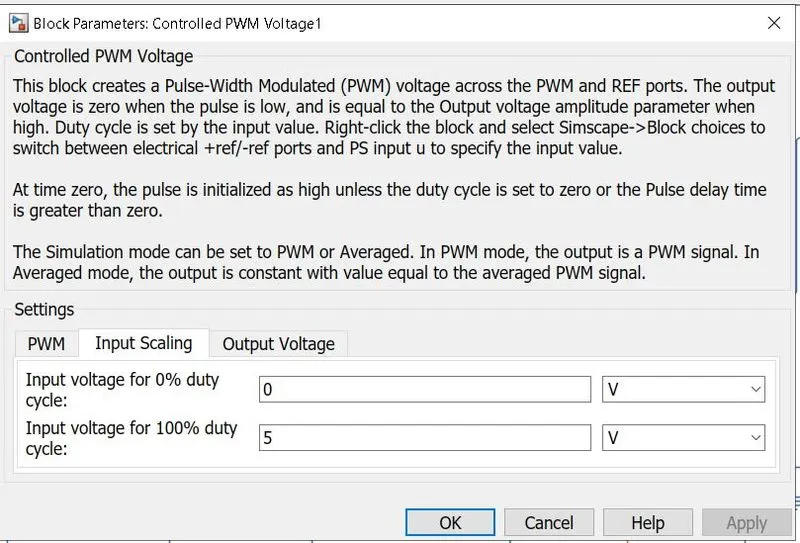
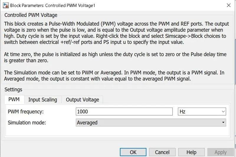
Controlled voltage source:

The Controlled Voltage Source block converts a Simulink input signal into an equivalent voltage source. The generated voltage is driven by the input signal of the block. You can initialize the Controlled Voltage Source block with a specific AC or DC voltage.

The block represents an ideal voltage source that is powerful enough to maintain the specified voltage at its output regardless of the current passing through it. The output voltage is V = Vs, where Vs is the numerical value presented at the physical signal port.

Current sensor:

The Current Sensor block represents an ideal current sensor, that is, a device that converts current measured in any electrical branch into a physical signal proportional to the current. Connections + and – are electrical conserving ports through which the sensor is inserted into the circuit.

3)Vehicle Dynamics/Drive Train Plant:

Vehicle dynamics subsystem is simply the vehicle body working to the given task. It has wheels, input to the wheels, output of the wheels, road conditions, surrounding conditions, load onthe vehicle etc.

Vehicle body:

The vehicle body block takes normal load on front wheel and rear wheels, road inclination, wind speed, force developed by tyres etc. into consideration and calculates vehicle speed.Represents a two-axle vehicle body in longitudinal motion. The block accounts for body mass, aerodynamic drag, road incline, and weight distribution between axles due to acceleration and road profile. The vehicle can have the same or a different number of wheels on each axle. Optionally include pitch and suspension dynamics or additional variable mass and inertia. The vehicle does not move vertically relative to the ground.

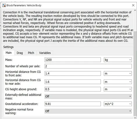
Connection H is the mechanical translational conserving port associated with the horizontal motion of the vehicle body. The resulting traction motion developed by tires should be connected to this port. Connections V, NF, and NR are physical signal output ports for vehicle velocity and front and rear normal wheel forces, respectively. Wheel forces are considered positive if acting downwards. Connections W and beta are physical signal input ports corresponding to headwind speed and road inclination angle, respectively. If variable mass is modeled, the physical signal input ports CG and M are exposed. CG accepts a two- element vector representing the x and y distance offsets from vehicle CG to additional load mass CG. M represents the additional mass.If both variable mass and pitch dynamics are included, the physical signal port J accepts the inertia of the additional mass about its own CG.

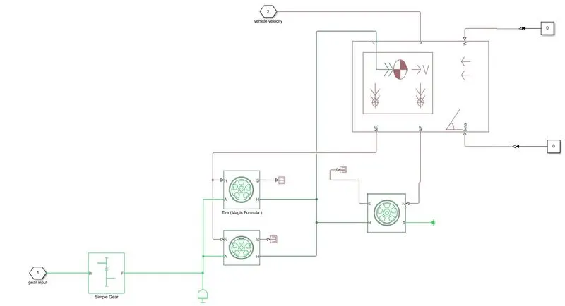
Tyres:

Tyre block represents the longitudinal behavior of a highway tire characterized by the tire Magic Formula. The block is built from Tire-Road Interaction (Magic Formula) and Simscape Foundation Library Wheel and Axle blocks. Optionally, the effects of tire inertia, stiffness, and damping can be included

Connection A is the mechanical rotational conserving port for the wheel axle. Connection H is the mechanical translational conserving port for the wheel hub through which the thrust developed by the tire is applied to the vehicle. Connection N is a physical signal input port that applies the normal force acting on the tire. The force is considered positive if it acts downwards.

Connection S is a physical signal output port that reports the tire slip. Optionally expose physical signal port M by setting Parameterize by to Physical signal Magic Formula coefficients.Physical signal port M accepts a four element vector corresponding to the B, C, D, and E Magic Formula.

Simple gear:

Represents a fixed-ratio gear or gear box. No inertia or compliance is modeled in this block. You can optionally include gear meshing and viscous bearing losses. Keeping the gear box has a gear ratio of 5 for this model.

Connections B (base) and F (follower) are mechanical rotational conserving ports. Specify the relation between base and follower rotation directions with the Output shaft rotates parameter. Optionally include thermal effects and expose thermal conserving port H by right-clicking on the block and selecting Simscape block choices to switch between variants.From this block the gear related variables are changed.

The output of the gear is given to the wheels. The normal force of the vehicle is also given to the tires as input. Tire slip is not considered in the simulation. Tyre generates the force to move the vehicle. This force is given to the vehicle body block.Vehicle speed is the ultimate output of this system.

4)Battery SubSystem:

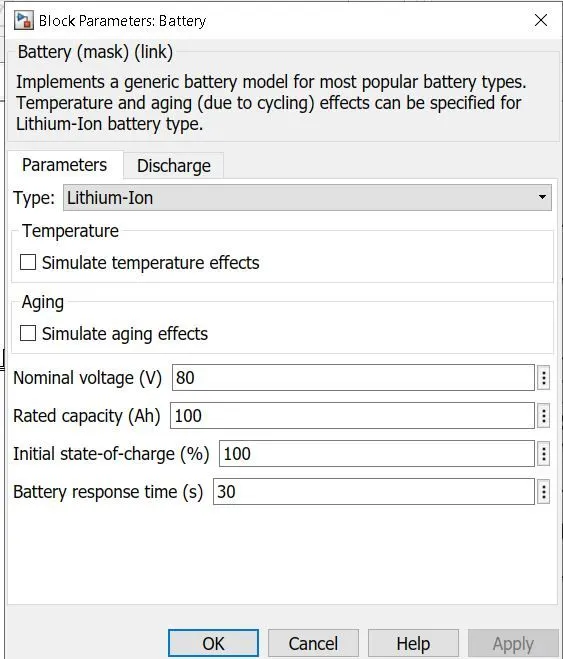
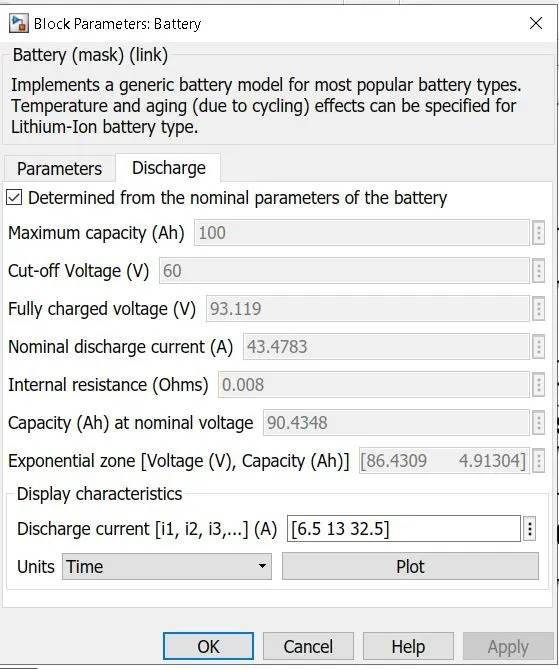
The battery used is a lithium ion battery of 80V and 100Ah capacity. The output of the battery is its current, SOC, and voltage. A controlled current souce drives the battery to charge and discharge. The input for this controlled current source is the current from the Power controller block.

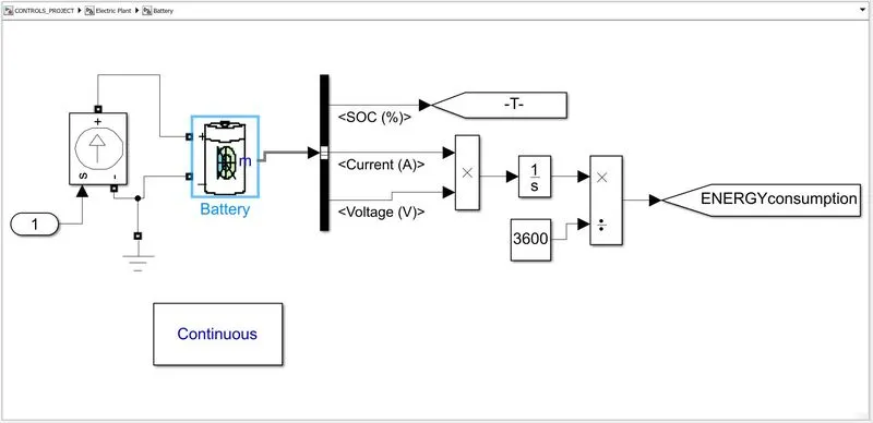
Battery:

Controlled current source:

The Controlled Current Source block converts the Simulink input signal into an equivalent current source. The generated current is driven by the input signal of the block. The positive current direction is as shown by the arrow in the block icon.The block represents an ideal current source that is powerful enough to maintain the specified current through it regardless of the voltage across it. The output current is I = Is, where Is is the numerical value presented at the physical signal port.

5)Longitudinal Driver/Controller:

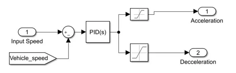
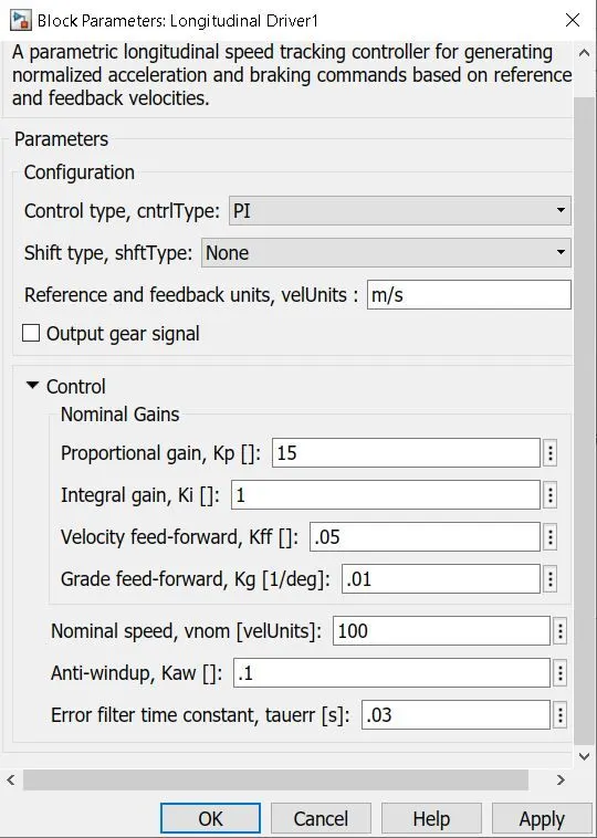
It is a simulated driving environment which follows the velocity input or This works based on the velocity reference(Vref) and velocity feedback (Vfb) as inputs, it’s a speed tracking controller and generates acceleration and braking commands as output to the controller. Longitudinal driver acts in such away that the difference between the velocity reference and velocity actual is minimised.From this block the variables can be changed like changing control type

This subsystem compares the input speed and the vehicle speed. If the output is positive speed accelerating command is given from the controller. If the output is negative, deceleration command is given from the controller output. If we use PID controller then the output is controlled by saturation blocks by giving the upper and lower limits. The PID controller is tuned and is a continuous time based in this model we have used PI Controller.

6)Drive Cycles:

Drive Cycles:

A driving cycle is a series of data points representing the speed of a vehicle versus time. They are standards of testing vehicles in order to validate their performance. Drice cycles are made

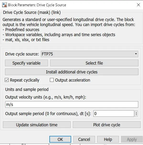
from vehicle travelling data. They are categorized in different types as for urban drive cycles, FTP cycles, WOT etc. We are usign two standard drive cycles here.

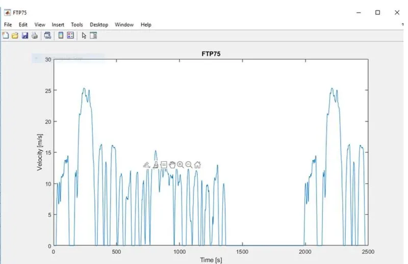
1. FTP75(2474 seconds):

The Federal Test Procedure (FTP) is composed of the UDDS followed by the first 505 seconds of the UDDS. It is often called the EPA75. The dynamometer portion of the test procedure has a very complex timeline of events.

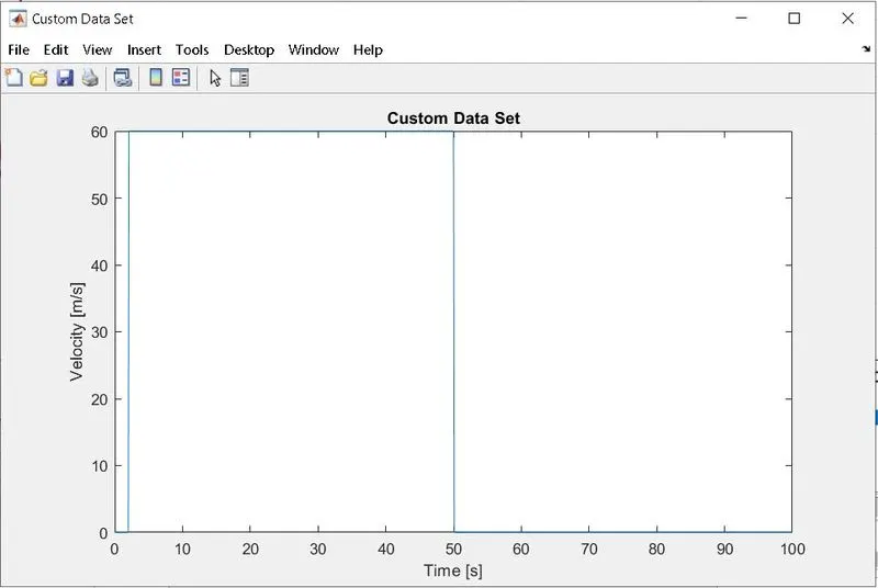
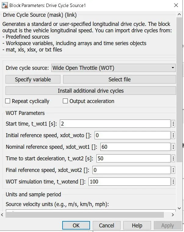
2. WOT(wide open throttle)100 seconds:

Generates a standard or user-specified longitudinal drive cycle. The block output is the vehicle longitudinal speed.

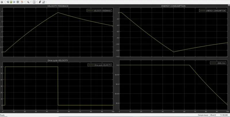
Zero for first 2 seconds, 60m/s for 2 to 50 seconds and zero from 50 to 100 seconds.

3. User defined cycle using signal builder:

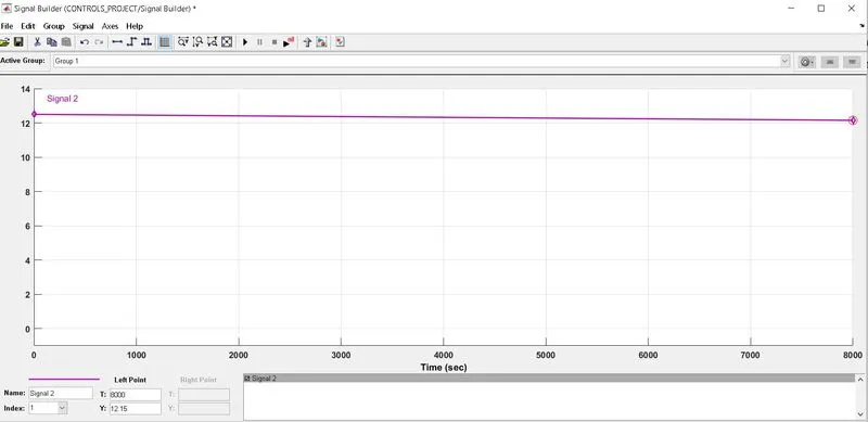
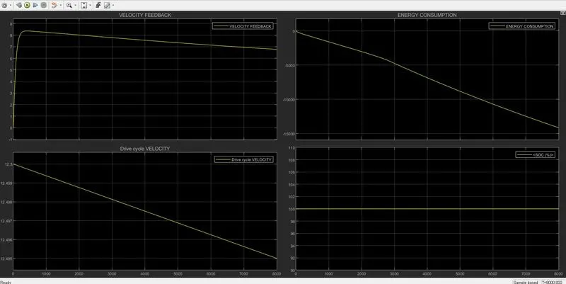
This cycles has a constant speed of 45kmph or 12.5m/s for 8000 seconds. The reason of the time being 8000 seconds is that the vehicle will take 8000 seconds for completing 100km ride at 45kmph speed.

OUTPUT RESULTS:

1)FTP75(2474 seconds):

Input speed/Drive cycle velocity VS output speed/Velocity Feedback:

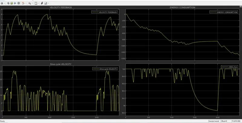
The modelled rickshaw efficiently follows the input drive cycle it has obtained as output according to the FTP 75 drive cycle and the nature followed by both are same and it can be tested for many drive cycles by selecting in the drive cycle block. The highest speed is 8Km/hr acheived from the velocity feedback output while following the input drive cycle.

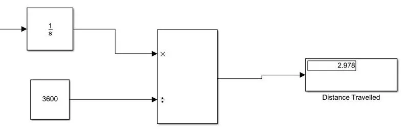
It has travelled a distance of 3Km by the used 80V battery capacity,if we increase the battery capacity to higher levels we can travel more distance.

State of charge(SOC):

SOC was constant when rickshaw was at rest. There is also regeneration seen and rise of SOC whenever speed was reduced or braking was needed. Here the SOC is reducing whenever the vehicle is accelerating because of the current drawn by the motor from the battery and SOC is improved whenever the vehicle is decelerating because of the current supplied by the motor to the battery. The minimum SOC level here is 98.7 .

Energy Consumption:

Energy consumption depends on the drive cycle nature or vehicle driving behaviour and road conditions and other factors more energy is consumed when the vehicle travels more distance with many variations in speed and viceversa.

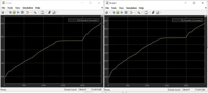
Controller/H- Bridge temperature Indicated with PS-Simulink Converter 2 output result:

Temperature of controller rises when the vehicle is running and is constant when it stops. Temperature increases from start till the end of drive cycle is 342kelvin which is the difference in rise from 298 - 640 kelvin.

Motor temperature Indicated with PS-Simulink Converter 1 output result:

The motor temperature profile is similar to controller temperature profile both are increasing when the vehicle is in motion Just the magnitude is different. Motor temperature rised to 500 kelvin from 298 kelvin.so,the difference in the rise is less than than the controller temperature i.e 202kelvin.

This rise of temperature should be controlled. It can be concluded that cooling medium is necessary for this powertrain in order to be efficient and long life. And whenever the vehicle stops we can see the saturation of temperature for both motor and controller at time period from 1200 - 2000 sec.

2.WOT(wide open throttle)100 seconds:

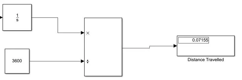
With the WOT drive cycle implemented the distance travelled is 0.07155Km, both the Input(drive cycle velocity) and output velocities(feed back velocity) are following and the nature is the same . From the feed back velocity graph the highest speed acheived is 3.8Km.

State of charge(SOC):

SOC was constant when rickshaw was at rest. Slight reduction from 100 %-99.8 % because of very less drive cycle time.

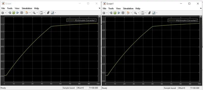
Controller/H- Bridge temperature Indicated with PS-Simulink Converter 2 output result:

Temperature of controller rises when the vehicle is running and is constant when it stops. Temperature increases from start till the end of drive cycle is 29kelvin which is the difference in rise from 298 - 327 kelvin. This rise in temperature is negligible.

Motor temperature Indicated with PS-Simulink Converter 1 output result:

Motor temperature rised to 312 kelvin from 298 kelvin.so,the difference in the rise is less than than the controller temperature i.e 14kelvin which is negligible. Because of less drive cycle time the temperature is increase is very less.

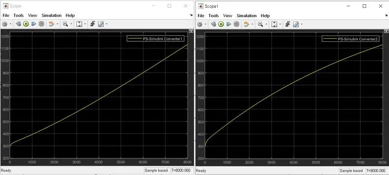
3.User defined cycle using signal builder:

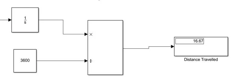
The distance acheived by using this drive cycle is 17Km,both the Input(drive cycle velocity) and output velocities(feed back velocity) are following and the nature is the same . From the feed back velocity graph the highest speed acheived is 8.2Km.

State of charge(SOC):

SOC was alomost unchanged till the end of the drive cycle this is because the vehicle is continuosly running at constant speed throughout the drive cycle and the charging is constantly provided to the battery.

Controller/H- Bridge temperature Indicated with PS-Simulink Converter 2 output result:

Temperature increases drastically from start till the end of drive cycle is 802kelvin which is the difference in rise from 298 - 1100 kelvin. This rise in temperature is negligible.

Motor temperature Indicated with PS-Simulink Converter 1 output result:

Temperature increases drastically from start till the end of drive cycle is 802kelvin which is the difference in rise from 298 - 1100 kelvin. This rise in temperature is negligible.

This very high increase in temperature is because vehicle is continuosly running at constant speed throughout the drive cycle with out any stops in between. It can be concluded that cooling medium is necessary for this powertrain in order to be efficient and long life.

CONCLUSION:

Hence Created a detailed MATLAB model of an electric rickshaw (three wheel passenger vehicle) by using Lithium ion battery and Rear wheels driven by PM brushed type dc motor.

Obtained all the Results For three standard driving cycles like FTP75,WOT,Manually drive cycle using signal builder plotted the energy consumption, temperature rise of motor and controller for 100 km constant speed driving at 45 kmph.