Final Project: Electric Rickshaw modelling

ANSWER : 

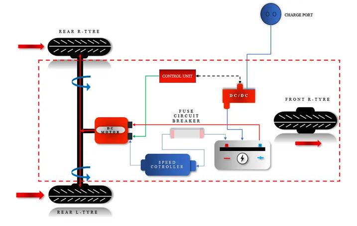
Electric E-Rickshaw is also known as electric tuk-tuk, e-rickshaw and auto which are going more popular after 2018 in Indian market. This E-rickshaw is best alternative of petrol/ CNG auto rickshaw and human or horse pulled rickshaws because of their low fuel cost, zero emissions and less human efforts.

The electrical system used in Indian version is 48VDC can run 90– 100 km/full charge, top speed 25 km/hour and this electric motor power ranging from 650-1400 Watts; the battery takes 8–10 hrs to become fully charged. Basic seating capacity is driver plus 4 passenger total 5 persons. 

MATLAB MODLE :

 

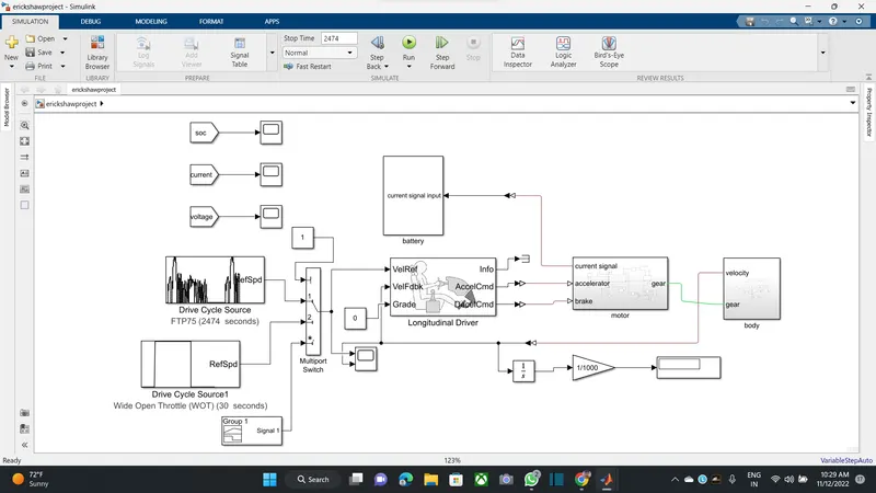
Full Model Parameter:

Drive cycle:

 

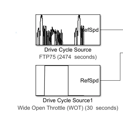
Generate a standard or user specified longitudinal drive cycle. 

MODELLING OF VEHICLE BODY SYSTEM: 

 

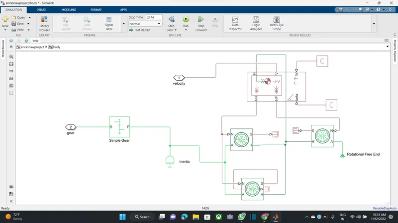
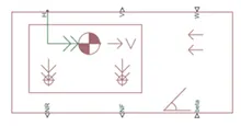
The above figure highlights the vehicle body for electric rickshaw which is having rear axle drive. The Vehicle Body block represents a two-axle vehicle body in longitudinal motion.

The block consists of body mass, aerodynamic drag, road incline, and weight distribution between axles due to acceleration and road profile. In optionally we can include pitch and suspension dynamics. 

1. NR: It is a physical signal output which is connected to the rear wheel axel. For this model, it is connected with a normal force of rear tire.
2. NF: It is a physical signal output which is connected to front-wheel axel and for this particular model it is connected with the normal force acting on a front-wheel tire.
3. Beta: Beta is basically a road incline angle. Here we can define a constant value for road angle inclination.
4. H: This port is a horizontal motion of the vehicle body. This connection will be connected with all four Hub of the wheel for finding the thrust generated by the tire.
5. V: This port is the vehicle longitudinal velocity.
6. W: It is a headwind speed. Basically, we will define a particular wind speed by adding constant block. 

 

• For setup of vehicle body just double click on the vehicle body and enter as per requirement.
• Here I have done some changes in vehicle configuration, Basically, I changed the vehicle mass, length and frontal area. 

TIRE MODELLING:

 

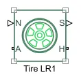
The Tire (Magic Formula) block models a tire with longitudinal behaviour given by the Magic Formula, an empirical equation based on four fitting coefficients. The block can model tire dynamics under constant or variable pavement conditions.

The Tire (Magic Formula) block models the tire as a rigid wheel-tire combination in contact with the road and subject to slip. When torque is applied to the wheel axle, the tire pushes on the ground (while subject to contact friction) and transfers the resulting reaction as a force back on the wheel. This action pushes the wheel forward or backwards. If you include the optional tire compliance, the tire also flexibly deforms under load. 

• N: Normal force acting on the tire and connected with NR of the vehicle body.
• S: Slip between the tire and road and connected with Goto block
• H: Hub and it is used to find the thrust created by the tire and it is connected with H input of vehicle body also including all four Hub of the wheel.
• A: Axel and rear axle are connected with the (Simple Gear) final drive system and the front axle is connected with the left and right wheel. 

INERTIA:

 

So here the inertia value is 0.01 kg×m^2 and this block is connected with rear axle and (Simple Gear) final drive ratio to find the inertia because axel and gear are a mechanical rotating device. 

SIMPLE GEAR:

 

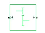
Simple Gear is a Final drive ratio which is a gearbox that constrains the connected driveline axes of the base gear and the follower gear.

B: The output B, base gear is connected with the input of DC motor R. It is a Rotational mechanical conserving port.

F: The output of F, follower gear is connected with the rear axle. It is also a Rotational mechanical conserving port.

CONFIGURATION BATTERY AND SOC:

 

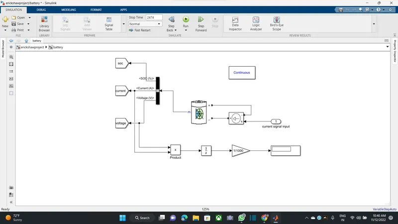
battery:

 

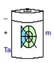
The circuit parameters can be modified to represent a specific battery type and its discharge characteristics. A typical discharge curve consists of three section .

Controlled Current Source :

The Controlled Current Source block converts the Simulink input signal into an equivalent current source. The generated current is driven by the input signal of the block. The positive current direction is as shown by the arrow in the block icon.

We can initialize the Controlled Current Source block with a specific AC or DC current. If we want to start the simulation in steady state, the block input must be connected to a signal starting as a sinusoidal or DC waveform corresponding to the initial values.

• Double click controlled current source and from drop down menu of measurement select current.
• Signal output will connect with scope by adding current signal to it.
• (+) terminal will connect with battery (-) terminal.

BUS Selector:

The Bus Selector block outputs the signals you select from the input bus. The block can output the selected elements separately or in a new virtual bus.

• Here just we have mange the output and connect with different Scope Block

PowerGUI

The powergui block allows us to choose one of these methods to solve your circuit:

• Continuous, which uses a variable-step solver from Simulink
• Discretization of the electrical system for a solution at fixed time steps 
• Continuous or discrete phasor solution

Motor:

 

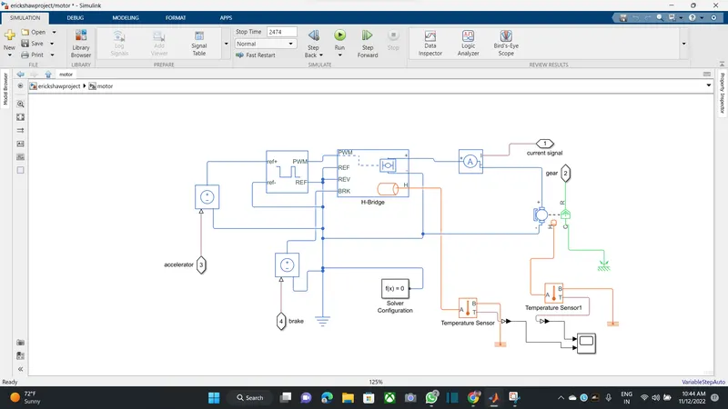
• PWM: Pulse-width modulated signal.
• REF: Reference, it is an electrical conversing port associated with the floating zero volts.
• REV: Reverse, it is an electrical conserving port associated with the voltage that controls when to reverse the polarity of the H-Bridge block output.
• BRK: BRK, it is an electrical conserving port associated with the voltage that controls when to short circuit the H-Bridge block output.

Here PWM output port is connected with PWM input port of controlled PWM voltage. The REF and REV port are connected with REF port of controlled PWM voltage port. The BRK port is connected with a controlled voltage source.

The positive (+) terminal is connected with the positive (+) port of current sensor and negative (-) port is connected with the negative (-) port of DC motor.

Thermal port (H) is connected with temperature sensor to measure the temperature of controller. 

CONTROLLED PWM VOLTAGE:

 

• ref+ — Positive terminal, this port is a positive electrical reference and connected with controlled voltage source positive terminal.
• ref- — Negative terminal, this port is a negative electrical reference and connected with the negative terminal of the controlled voltage source.
• PWM — Pulse-width modulated signal, this port is electrical reference port and connected with PWM port of H-Bridge.
• REF — Floating zero-volt reference, this port is connected with REF and REV of H-Bridge port. 

LONGITUDINAL DRIVER:

 

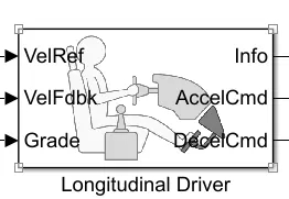
• VelRef: Reference vehicle velocity is connected with speed result block. Its unit is m/s.
• VelFdbk — Longitudinal vehicle velocity is connected with integrator block for continuous-time integration of VelFdbk signal.
• Grade — Road grade angle is connected with constant block so that we can use our specific value, here the value is 0 which I used.
• Info — Bus signal, Here I used this signal to terminate the signal block, basically it’s an output port.

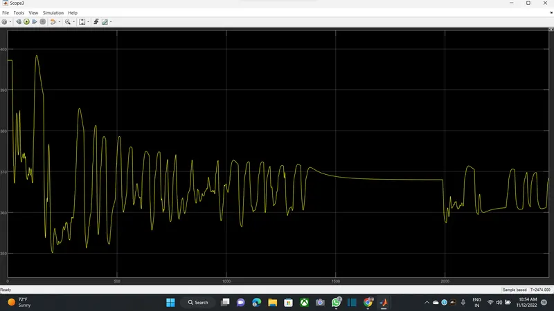
RESULTS :

 

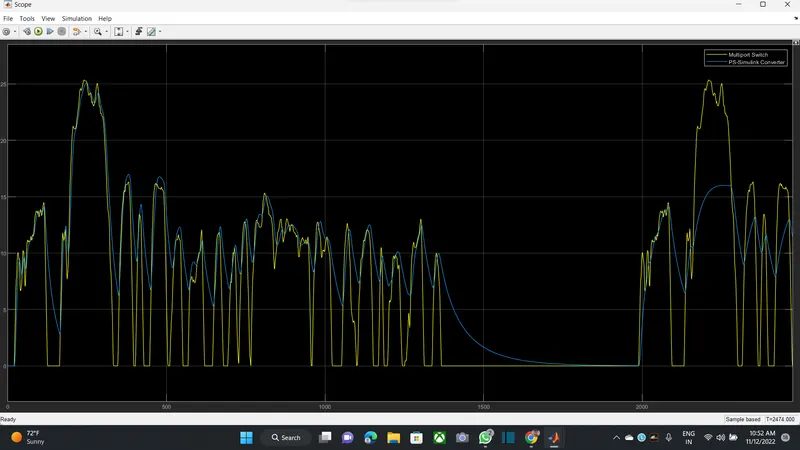
soc:

 

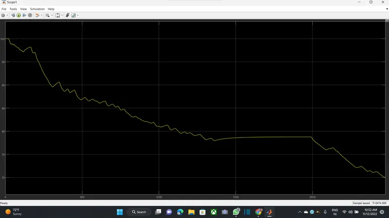
current:

 

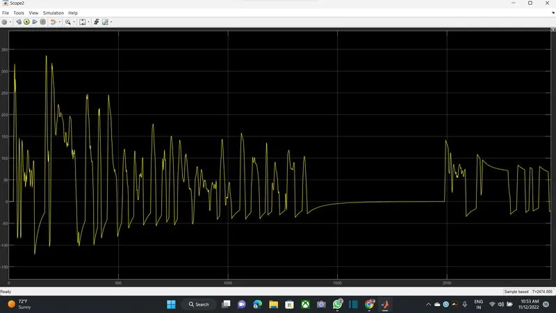
voltage: