Final Project: Electric Rickshaw modelling

Final Project

Electric Rickshaw modelling

Create a detailed MATLAB model of an electric rickshaw (three-wheel passenger vehicle) as per details below:

Rear wheels driven by PM brushed type motor

Assume efficiency points of motor controller and motor

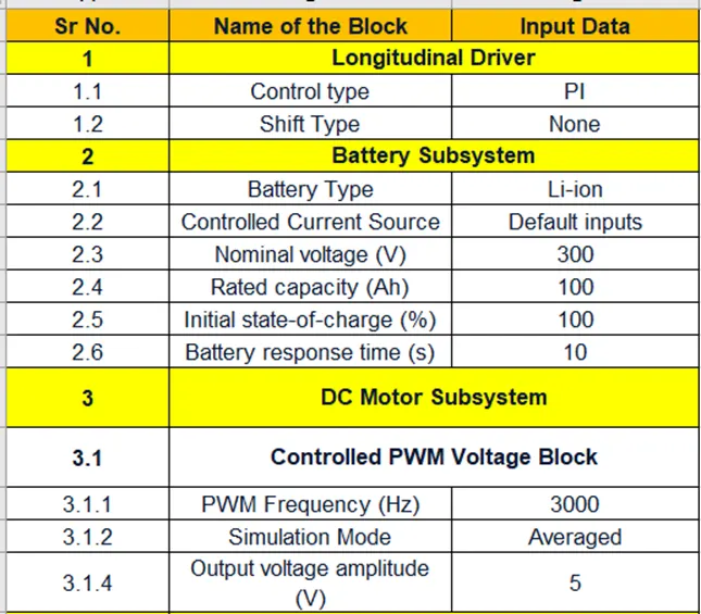
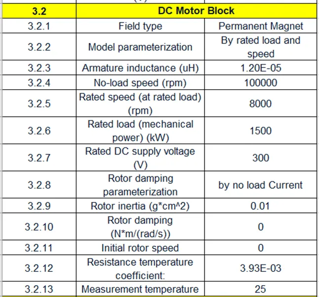
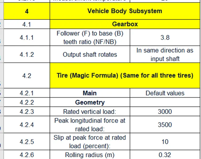
Make an excel sheet of all input and assumed data

Results: For any three standard driving cycles show energy consumption, temperature rise of motor and controller for 100 km constant speed driving at 45 kmph.

Answer:

ABSTRACT:

Using a PM brushed type DC motor and an appropriate Lithium-Ion battery for the motor, we will construct the MATLAB model of the ELECTRIC RICKHAEW in this project. We shall first discuss what an electric Rickhaew is, how it functions, and its advantages. A real EV RICKHAEW model is then created in SIMULINK using the appropriate blocks from the powertrain block set. My major goal is to see how well my Rickheaw operates over any three typical driving cycles, which include measuring the amount of energy used, the temperature rise of the motor, and controller during a 100-kilometer trip at a constant 45 kmph. compared my Simulink model to the Mahindra e-Rickhaew.

OBJECTIVES:

According on the information below, build a thorough MATLAB model of an electric rickshaw (a three-wheeled passenger vehicle):

1. Driven by a PM brushed type motor, the back wheels
2. Consider the motor controller and motor's efficiency points.
3. Compile all input and suppositional data into an excel sheet.
4. Results: Show energy usage, motor and controller temperature rise for any three normal driving cycles for a 100 km drive at 45 kmph.

METHODOLOGY:

• The battery, motors, and controller that make up an electric car are used to produce propulsion power.
• To construct any vehicle, we must first determine its propulsion power before choosing a motor.
• Lastly, we want to rely on the total battery capacity and then battery capacity is chosen depending on the motor rating or operational range and no km/charge. Therefore, the vehicle engineer's design process must resemble the following:
• Determine the necessary propulsion power.
• What motor is the most appropriate for such propulsion power?
• Then, according to the range, kind of battery and battery size

INTRODUCTION:

• Electric tuk-tuks, e-rickshaws, and autos are other names for electric e-rickshaws, which are becoming increasingly well-known in the Indian market after 2018. Due to its cheap fuel costs, lack of pollutants, and minimal human effort, this E-rickshaw is the perfect replacement for petrol/CNG car rickshaws and human or horse-pulled rickshaws.
• With a 48VDC electrical system, the Indian version's electric motor has a power range of 650-1400 Watts and can go up to 90-100 km per full charge with a peak speed of 25 km/h. The battery needs 8 to 10 hours to charge completely. The minimum seating capacity is for 5 people, including the driver.
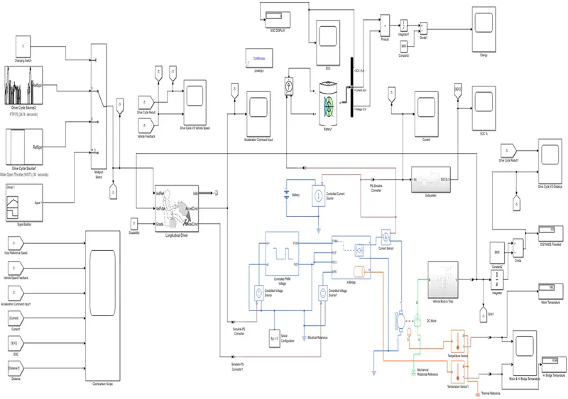
• Basically, CREO and MATLAB Simulink are used here to build the e-rickshaw. The battery, driving cycle, regulated, DC motor, vehicle body, and transmission system are the primary building components of the developed electric rickshaw. Drive cycle is the human input that determines how he will drive his real cycle. Drive cycles like FTP75, WOT, or Excel can be used.
• This project's primary goals include measuring the driver's speed, the motor and controller's temperature, the state of charge (SOC), and the vehicle's distance travelled. The battery's level of charge is estimated by a SOC block, and for each of the three Drive cycles, distance is computed using the speed and duration parameters.

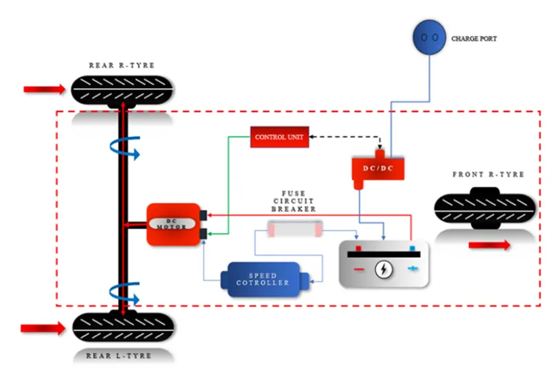
Design and Construction:

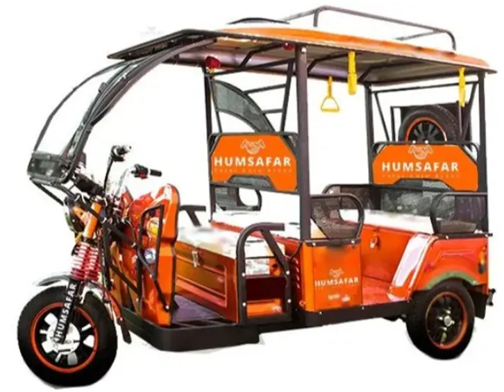
These rickshaws feature a three-wheeled, M.S. (Mild Steel) tubular chassis with a differential system at the back wheels. The motor is a brushless DC motor that is mostly made in China and India. In Bangladesh, a 60V electrical system is utilised, compared to 48V in India. The most widely used Chinese version's body is made of very thin iron or aluminium sheets. Because of their strength, longevity, and low maintenance requirements, vehicles built of fibre are extremely well-liked, particularly in India.

There are many different body types, including freight carriers, passenger cars without roofs, and full-bodied cars with windshields for the convenience of the driver. There is a controller unit included. They are priced according to the amount of voltage and current they produce as well as the quantity of MOSFETs (metal oxide field-effect transistors) that are employed. The typical battery is a lead-acid battery with a lifespan of 6 to 12 months. Rarely are deep cycle batteries made for electric cars employed. The weight of the electric automobile has also consistently presented design challenges.

WORKING:

As soon as the motor becomes excited, the input drive cycle begins. and it delivered cycles are documented for the initial input cycle and ultimate output drive cycle comparison. The same is inputted to the longitudinal driver, which decodes the command and converts it to machine language before moving on to the motor controller, which generates the pulses (commands are carried out with the aid of controlled PWM voltage), and the H-Bridge, which accepts multiple inputs and delivers the command signal to the motor with the aid of voltage and current sensors.

The current and voltage fluctuation is seen based on the signals. The transmission system, which is really the practical element, receives signals from the controlled motor after that. A basic gear coupled to the wheels (or tyres) provides acceleration, deceleration, braking, and reverse driving, and as a result, the vehicle body responds as necessary.

The end velocity is noted and will afterwards be contrasted with the input velocity.

In addition, battery performance is tracked concurrently in order to estimate the vehicle's efficiency over the course of the voyage.

PROCEDURE:

Model for the Vehicle Body Subsystem:

• The motor will generate the rotational output that the car body and gearbox will receive. Here, the gear system uses the rotational output to keep the transmission's speed constant from the motor to the tyres without reducing it.
• Here is a schematic showing the relationship between the transmission system and the vehicle's body. In the primary design, the term "transmission system" is used.
• I designed a rear-wheel drive gearbox arrangement in this instance.

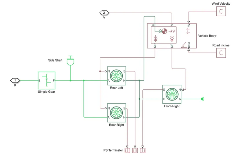
• The circuit depicts that the gear is linked to the rear wheels and the front tyre is free to rotate. As a result, the vehicle advances. The gear output is sent to the axels of the rear tyres. The tyres' normal force, N, is applied to the car body's normal force port.

• The H-Hub, S-Tire Slip, N-Normal Force, A-Axel Connection, Wind Velocity, and Inclination Angle of the vehicle body. The car body is joined to the tyre hub as a single node.

• The beta-inclination angle is connected to another constant block, and the vehicle body wind velocity is connected to another constant block. These constant blocks allow us to assign the wind velocity and inclination angle as needed. The output port for velocity allows us to determine the vehicle's current speed. The distance travelled and state of charge are calculated by subtracting the velocity.

Vehicle Body Parameters:

Modifications are made to the vehicle's body mass, center of gravity distances, and aerodynamic drag parameters.

With other variable settings set to their default states, pitch dynamics are maintained ON.

Tire:

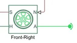
Represents a highway tire's longitudinal behaviour as defined by the tyre magic formula. The tire-road interaction (magic formula) and Simscape Foundation Library Wheel and Axle blocks are used to construct the block. The impacts of tyre stiffness, damping, and inertia are optional.

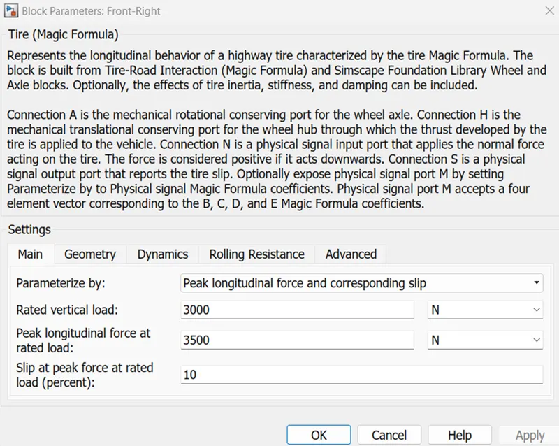
The mechanical rotational conserving port for the wheel axle is Connection A. The mechanical translational conservation port for the wheel hub, or Connection H, is where the tire's generated thrust is transferred to the car. The physical signal input port known as Connection N applies the tire's typical force. If the force acts downhill, it is seen as positive.

The physical signal output port Connection S reports the tyre slip. Set Parameterize by to Physical signal Magic Formula coefficients to optionally reveal physical signal port M. The B, C, D, and E coefficients of the Magic Formula are represented by a four element vector that may be input into physical signal port M.

Gear:

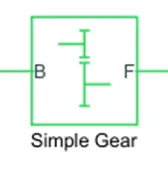
Represents a gear or gear box with a set ratio. In this block, neither inertia nor compliance are represented. The inclusion of viscous bearing losses and gear meshing is optional.

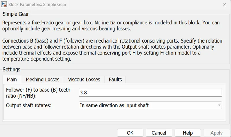
• Base and follower connections B and F are mechanical rotational conserving ports. Use the Output shaft rotates parameter to specify how the base and follower rotation directions relate to one another.
• By choosing Simscape block options from the context menu when you right-click on the block to choose between the two options, you may optionally add thermal effects and reveal thermal preserving port H. The input and output shafts both revolve in the same direction.
• The follower is attached to the rear wheel axle, and the base is connected to the motor shaft.

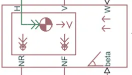
In a specific block

NR: The rear wheel axel is coupled to a physical signal output. This model connects it to the typical force of the rear Tyre.

NF: For this particular model, it is tied to the normal force acting on a front-wheel Tyre and is a physical signal output connected to the front-wheel axel.

Beta: A road inclination angle can be thought of as beta. Here, we can define a constant value for the inclination of the road angle.

H: The vehicle body is moving horizontally in this port. For the purpose of determining the thrust produced by the Tyre, this connection will be connected to each of the four-wheel hubs.

V: The vehicle's longitudinal velocity can be found here.

W: The speed is in the headwind. In essence, we will add constant blocks to establish a specific wind speed.

Simply double-click the car body to configure it according to your needs.

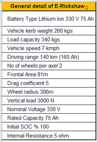
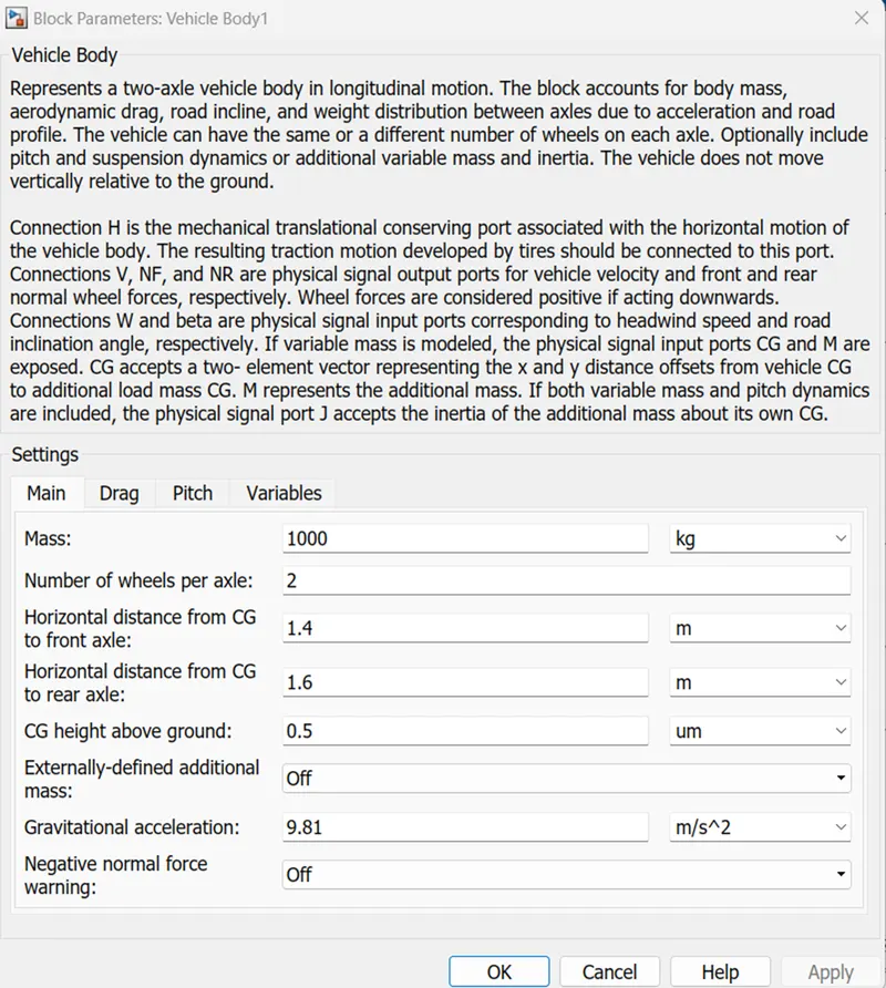
Here, I've made a few modifications to the vehicle's design. Specifically, I adjusted the vehicle's mass, length, and frontal area.

The vehicle's geometrical specifications are as follows:

PS – Terminator:

To end physical signal outputs, use this block. Physical signal output ports that aren't connected don't produce warnings, however connecting to a PS Terminator can show that the signal wasn't unintentionally left disconnected.

Main:

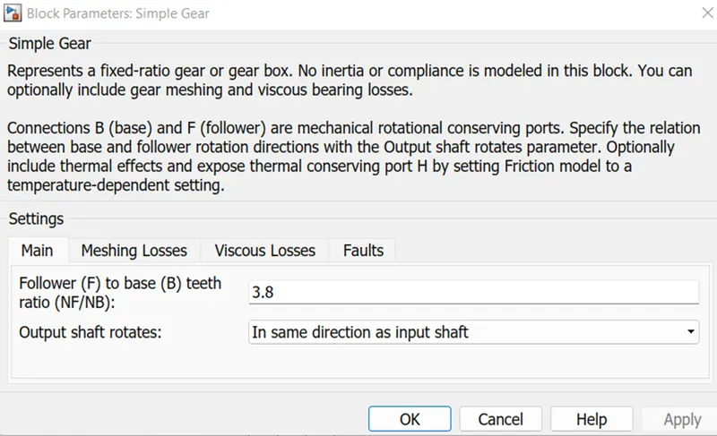
The follower to base teeth ratio, one of the key components of the basic gear, has been set to 3.8. Additionally, I have said that the output shaft should rotate parallel to the input shaft rather than in the opposite direction from the input shaft.

Meshing Losses:

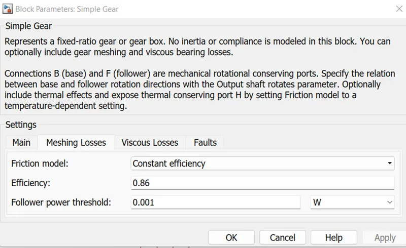
The friction model for the meshing losses I've chosen has an efficiency of 0.86 and a follower power threshold of 0.001W.

Inertia:(Side Shaft)

To give the proper mechanical rotational inertia for the straightforward gear block, an inertia block has been added to the workspace. This block only contains one mechanical rotational conserving port, and the block's positive direction is from the port to the reference point, which in this case would be a straightforward gear. The acceleration of inertia in a positive direction causes the inertia torque to act in that direction. Below is a diagram of the inertia block:

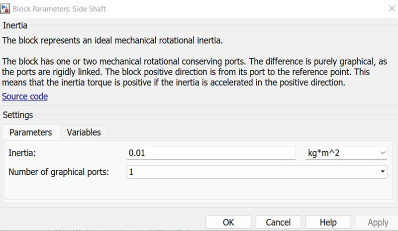
Only the inertia can be changed using the inertia block parameters, which is why the default value of 0.01 has been retained.

Slope & Wind

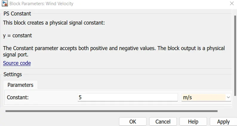
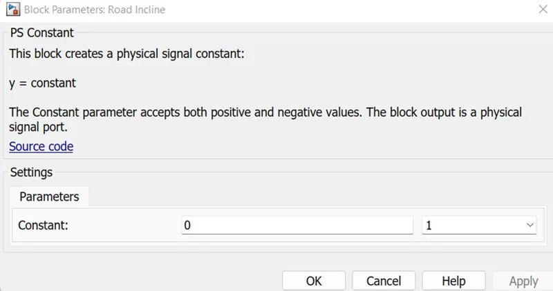
As previously noted, we may simulate the effects of wind resistance and road incline using the velocity block's "W" and "beta" ports, respectively. In order to simulate the effects of wind and road inclination on the motion of the car, I used a "PS - Constant" block in my model. I have a steady signal of 5 m/s for the wind effect, and this functions as a headwind, which is the opposite of the direction of motion. I have consistently signaled 0 for the road incline. The following graphics display the block settings for the wind and slope effects:

Motor & Power Converter Subsystem Model (Including Temperature Sensor):

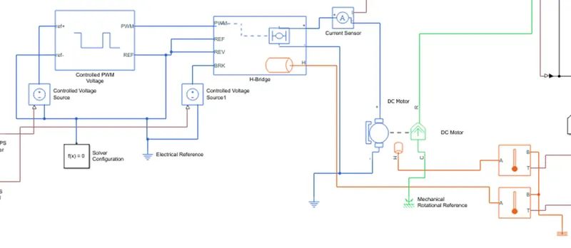
H-Bridge:

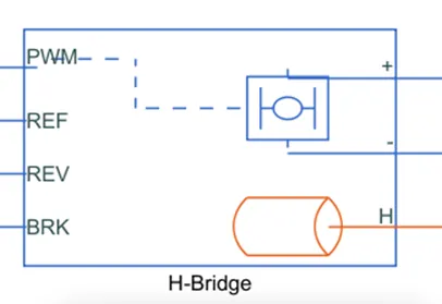
The H-bridge motor drive is illustrated by this block. The block may be operated in PWM or Averaged mode by the Controlled PWM Voltage block. If the PWM port voltage is higher than the Enable threshold voltage, the motor is operated in PWM mode.

The ratio of the on-time to the PWM period is determined in Averaged mode by dividing the PWM port voltage by the PWM signal amplitude parameter. The block applies an average voltage to the load that results in the right average load current using this ratio and assumptions about the load.

The Controlled PWM Voltage and H-Bridge blocks both require the same value for the parameter in Simulation mode.

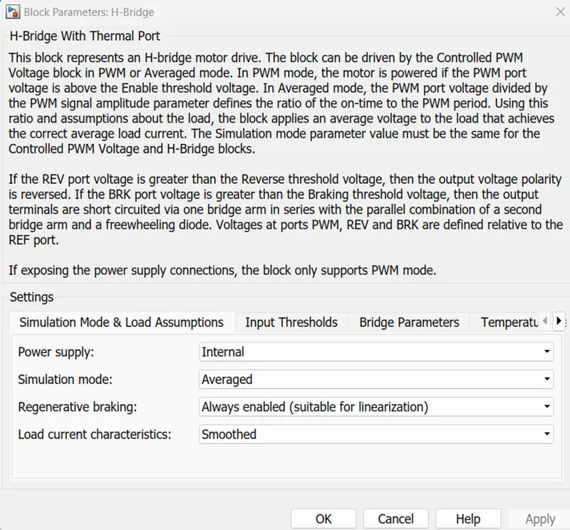
The output voltage polarity is reversed if the REV port voltage is higher than the Reverse threshold value. The output terminals are short-circuited through one bridge arm in series with the parallel pairing of a second bridge arm and a freewheeling diode if the BRK port voltage is higher than the braking threshold value.

The REF port serves as the reference point for the voltages at ports PWM, REV, and BRK. The block only supports PWM mode when the power supply connections are exposed.

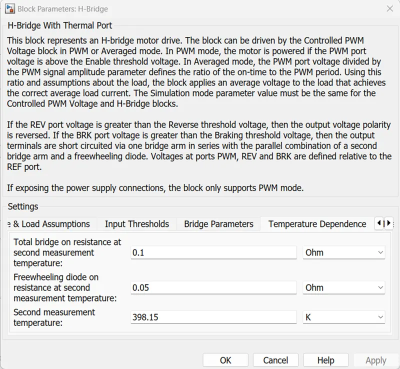
Thermal Port:

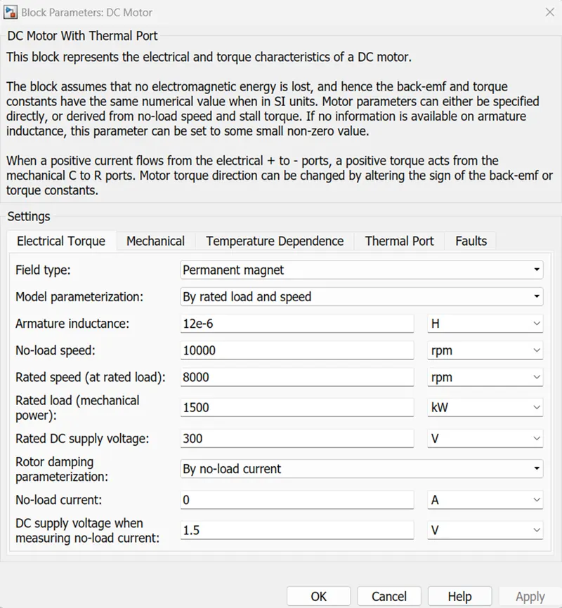
DC Motor:

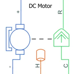
A thermal port to sense the motor's temperature is included in this block, which depicts the electrical and torque properties of a DC motor.

The back-emf and torque constants have the same numerical value when expressed in SI units because the block assumes that no electromagnetic energy is wasted. In addition to being directly provided, motor characteristics can also be obtained from stall torque and no-load speed. If no data on armature inductance is available, this parameter can be set to a negligible non-zero value.

Positive torque acts from the mechanical C to R ports when a positive current flow from the electrical + to - ports. By changing the sign of the back-emf or torque constants, the direction of the motor torque may be adjusted.

The longitudinal driver will provide information to the motor controller. Its duties include regulating the motor's speed and operating in accordance with the driver's input. PWM voltage generator and H-Bridge were the two key components of our mostly motor-controlled architecture.

A controlled voltage source block receives input 1 from a longitudinal driver's accelerator and passes it on to a controlled PWM voltage. Controlled PWM voltage will provide a PWM signal that will cause an H-bridge to produce the necessary voltage to drive a DC motor using the provided driver input.

Ground and the H-REF bridge's serve as the negative reference and REF, respectively, for the PWM voltage block. The H-bridge is a motor controller that only operates two IGBT components at once in response to the input of the signal from the PWM block. The components are arranged in the shape of an H.

This Hbridge's positive and negative terminals will output when there is a slowdown. Later, the DC motor and battery are linked to these negative and positive terminals. All of these parts are electrical simscape parts, hence they require a link to the solver configuration block in order to aid with simulation resolution.

Mechanical rotational reference block:

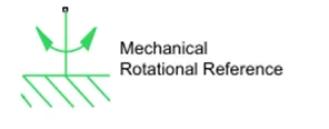
This block depicts a frame or a ground, which is a mechanical rotational reference point. Use it to link the rigidly attached mechanical rotational ports to the frame (ground).

Controlled PWM Voltage:

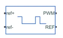
The H-Bridge block is then given a regulated pulse width modulated voltage using a "Controlled PWM Voltage" block. The block will feed into the same ports present on the H-Bridge block through its "PWM" and "REF" ports, which will output the PWM voltage. The output voltage is zero volts (V) if the pulse is low, and the output voltage is equal to the output voltage amplitude (300V) if the pulse is high.

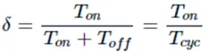
This block generates voltage pulses that depend on the duty cycle, which is the ratio of the time the switch is ON to the time it takes to complete one cycle (which is the time for which the switch is ON and OFF). The input of the regulated PWM voltage block controls the duty cycle.

The formula for duty cycle is provided by:

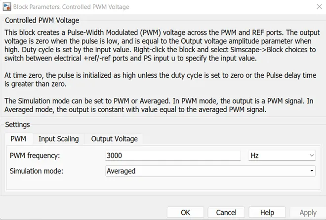
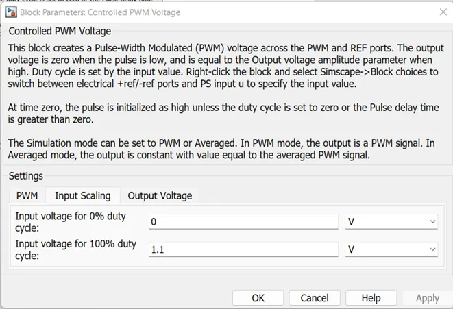
The PWM parameters are where most settings are made. All of the parameters in this case are left at their default settings. I have selected the "Averaged" simulation option, which generates and feeds the H-Bridge with voltage pulses of an average value. Similar to the H-Bridge block parameters, this will enable faster simulation times. The remaining values for "Input Scaling" and "Output Voltage" stay the same.

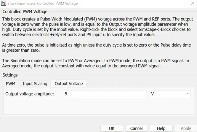
Here the Output Voltage is only 5 V, because the H- Bridge is a Semiconductor device so the less voltage is enough for that.

Electrical Reference:

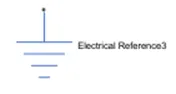
A grounding effect is produced for electrical circuits using the electrical reference block. There must be at least one electrical reference block in each model that has electrical or electronic components. Below is a diagram of the electrical reference block

We make use of this block twice in my EV model. The first step is to establish an electrical ground between the H-Bridge blocks and the controlled voltage source, regulated PWM voltage. The second one pertains to the battery system, which will be modelled later.

Controlled Voltage Source:

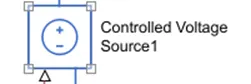
Because they need a controlled voltage source to supply the voltages to make the voltage pulses that must be sent into the H-Bridge, the input ports of the controlled PWM voltage block are still unconnected. I have the regulated voltage source block for this. This block is advantageous because it will supply the required voltage, which is strong enough to keep the output voltage constant regardless of the current flowing through it. Below is a diagram of this regulated voltage source block

Two regulated voltage sources have been applied in this model. The voltage for the vehicle's acceleration will come from one block, while its deceleration or braking will come from the other.

Solver Configuration:

In order to solve any essential equations in a model, the solver configuration block is used. In my example, I connected it to the H-Bridge block's "REV" port. The block that configures the solver is displayed below

Longitudinal Driver:

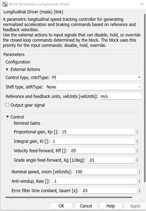
On the basis of two sets of data, the longitudinal driver block is utilized to send a controller normalized acceleration and deceleration signals. The reference velocity is represented by the first data set, and the feedback velocity by the second.

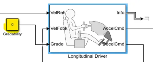
Below is a diagram of the longitudinal driver block:

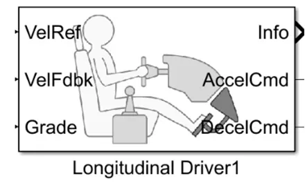
The ports on the longitudinal driver block are as follows:

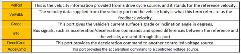
The longitudinal driving block has an easy-to-understand mechanism. The feedback velocity data from the vehicle body block is compared to the reference velocity data from a drive cycle source. The controlled voltage source will receive an acceleration command as an output if the reference velocity is higher than the feedback velocity. The output to another controlled voltage source is changed to a deceleration command if the reference velocity is less than the feedback velocity.

A Simulink - PS converter block was utilized to translate the acceleration and deceleration commands into output signals. When connecting a Simulink input signal to a physical signal, we must use this block. In this situation, the input signal is velocity data, which is logic data that we wish to transform to a physical signal, i.e., voltages to the controlled voltage source.

The picture below shows the longitudinal driver block parameters:

Below is a diagram of the Simulink to PS converter block:

Converts the Simulink input signal to a Physical Signal.

Grade:

A constant block with a constant value of 0 is linked to the longitudinal driver block's grade port. This prevents the simulation from modelling any road inclination.

The illustration below shows how this works:

Terminator: (For Info Point)

Made use of to "terminate" output signals. (Prevents notifications of disconnected output ports.)

Temperature Sensor:

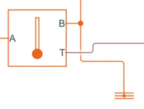
• H-Bridge and motor temperatures are measured using a temperature sensor.
• A thermal network's temperature is measured by this block. The sensor does not experience any heat flow. The temperature differential across the sensor is reported by the physical signal port T.
• When the temperature at port A is higher than the temperature at port B, the measurement is positive.

Solver Configuration:

Defines the simulation-related solver parameters.

Controlled Voltage Source:

The block is a representation of a perfect voltage source, capable of sustaining the desired voltage at its output regardless of the amount of current flowing through it. The physical signal port's displayed numerical value, Vs, determines the output voltage, which is expressed as V = Vs.

Battery and Soc Model:

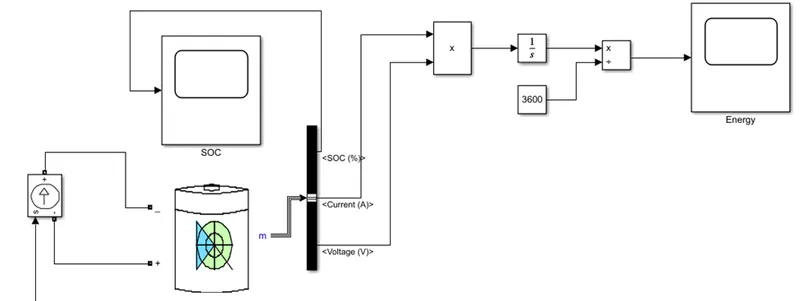
Battery:

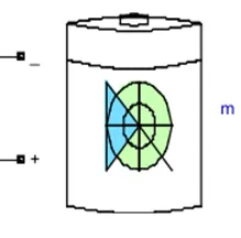
• A general dynamic model that depicts the most common types of rechargeable batteries is implemented by the battery block.
• Simply make the modifications I outlined above in battery configuration.
• Simply connect the battery's Ta input and the outside temperature.
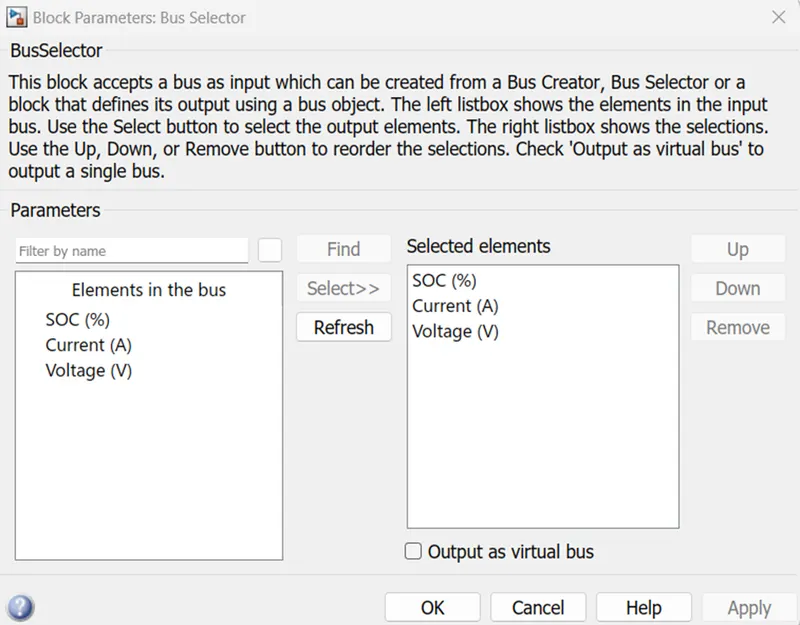
• BUS selector lock will be attached to "M."

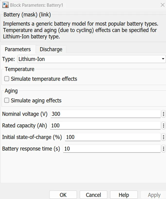
There are two stages for the battery: a charging stage and a discharging stage. 100Ah is the battery's capacity.

The battery's nominal voltage is 300 V, and the initial SoC is 100%.

The battery as a source of charge-dependent voltage and a series internal resistance described by:

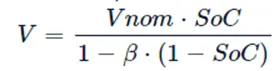
where Vnom is the nominal voltage and SoC is the state of charge. A user-defined data point [AH1,V1] is satisfied by the coefficient beta calculation.

The battery contains a positive and negative terminal that are connected to a voltage-controlled source, where the motor controller regulates the battery usage before passing it to the SOC block.

Battery State of Charge:

• The state of charge, or SoC, of a battery after a specific amount of travel or battery charge use by the vehicle.
• In the designed vehicle, the battery charge, or SOC, is calculated by giving it to the rate transition and then gaining where 1/(nominal battery capacity) then to a discrete-time integrator and it will get minus from the 1, as it is considered a 100% of battery and it is multiplied with 100 to get percentage of battery.
• The bulk of blocks are Simscape blocks, and the physical signal from a Simscape block is converted to a Simulink signal using a Physical to Simulink Converter.

BUS Selector:

The signals you choose from the input bus are output by the bus selector block. The block has two output options: a new virtual bus or the selected pieces output individually.

Just manage the output and connect to various Scope Blocks here.

Power GUI:

We can select one of these approaches to fix your circuit thanks to the powergui block:

Continuous, which makes use of a Simulink variable-step solver

Electrical system discretization for a solution at certain time steps

Discrete or continuous phasor solution

The powergui block additionally provides access to tools for sophisticated parameter design as well as tools for analysing simulation and steady-state findings.

We must build a subsystem using blocks named Rate transition, Gain, Discrete Time Integrator, Constant, and Sum in order to calculate the SOC (State of Charge).

Alternate Battery: (Connections)

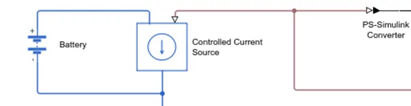
Battery:

The EV's energy source will be the battery, which will hold the electrical energy in DC form and supply it to the DC motor so it can run. The battery block in use just considers the fundamental characteristics.

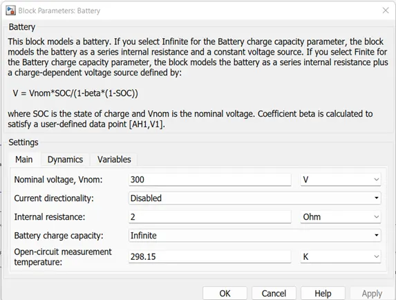
The nominal voltage, internal resistance, and battery charge capacity are all part of the battery block parameters, as can be seen. I've utilized a 300V nominal voltage, 2 Ohms of internal resistance, and an endless battery charge capacity. The nominal voltage is chosen so that it is more than enough to supply the DC motor and the H-Bridge blocks with voltage.

Controlled Current Source:

The block is a representation of a perfect current source, capable of sustaining the desired current through it independent of the applied voltage. I = Is, where Is is the numerical value displayed at the physical signal port, equals the output current.

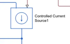
Send the input signals that correspond to the first input's shortened value through. Top to bottom, the inputs are numbered (or left to right). The control port is the first input port. Data ports make up the remaining input ports.

Current Sensor:

A device that transforms current sensed in any electrical branch into a physical signal proportionate to the current is represented by the block as an ideal current sensor.

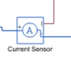
The electrical ports that the sensor is introduced into the circuit through are connections + and -. A physical signal port called Connection I outputs current value.

Current & SOC:

SOC, which stands for state of charge, is a measurement of the amount of charge that is currently present in a battery. A battery is said to be fully charged when it is at 100% charge, and totally discharged when it is at 0% charge. I want to monitor the battery's SOC and current in this EV model as the simulation is running. I've done this by using a scope block, which displays the output signal we want to measure as a plot against time. One scope was utilized for the current and the other for the SOC. We must utilize a "PS - Simulink converter" block in order to measure this.

Below is a diagram of the PS to Simulink converter block:

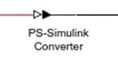
Translates the physical signal input into a signal produced by Simulink.

The conversion from the Physical Signal to the Simulink output signal is determined by the unit expression in the "Output signal unit" parameter, which must match or be commensurate with the unit of the Physical Signal.

SOC Subsystem:

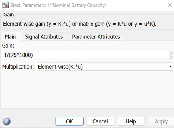
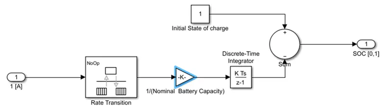
An intricate subsystem made of different building blocks was developed to gauge the battery's state of charge. The 'Rate Transition' block, which is the first block, manages data transfer between various rates and tasks. The signal from the rate transition block is then multiplied or divided using a "Gain" block. In this instance, the gain block will split the current signal by the battery's ampere rating, which has been assumed to be 80Ah times 3600. (seconds in one hour)

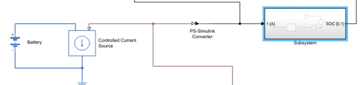
The current signal is then discretely integrated with respect to time using a "Discrete - Time Integrator" block. The battery's initial SOC is represented by a constant block. When running a simulation, I usually assume that the battery is fully charged, therefore I changed the constant block to have a value of 1, which stands for 100%. After that, operations like addition and subtraction are carried out using a "sum" block. The constant block indicating a 100% charge will be deducted from the signal from the "discrete time integrator" block. The connections between these parts are as follows:

The PS-Simulink converter block is then used to link these blocks with the battery circuit in a subsystem dubbed "SOC Estimate." The output signal of the current from the battery is shown using a scope block at the junction of the PS-Simulink converter block. The output signal of the SOC from the SOC subsystem is plotted using a different scope.

Vehicle Distance:

In order to calculate the distance, the vehicle has travelled based on the drive cycle data, I have utilized the scope block and mathematical operator block. In my model, the area under a velocity time graph indicates the distance travelled by an object. This indicates that the distance travelled is equal to the integral of the velocity with respect to time. In order to integrate the velocity signal output by the vehicle subsystem, I have created the integrator block.

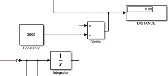
Integrator block:

I had to divide the integrated speed signal, which is expressed in kilometers per hour, by 3600 using the "Divide" block from the integrator block and a "Constant" block with a value of 3600. This will provide us with the kilometer-based distance travelled.

Constant block:

Output the constant specified by the 'Constant value' parameter

Divide Block:

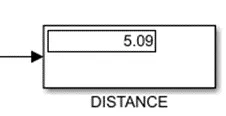
The simulation's 'Display' block is used to display the distance travelled.

Display:

This is the display block used to display the output values, here we calculated the total distance Travelled

Goto Block:

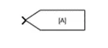
Send signals to ‘From’ blocks that have the specified tag

From Block:

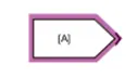
Receive signals from the ‘Goto’ block with the specified tag.

Reference Velocity (Drive Cycle):

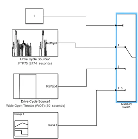
• Drive cycle has taken the role of the driver's actual driving style as the vehicle's input. In this case, I tested the vehicle's performance using three drive cycles. There will be high speed, low speed, and brake circumstances in these driving cycles.
• Different drive cycles, such as WOT and FTP75, exist. For this model, I utilized the WOT and manually produced FTP 75 drive cycle sources.

1) FTP75:

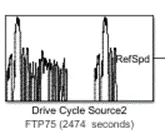
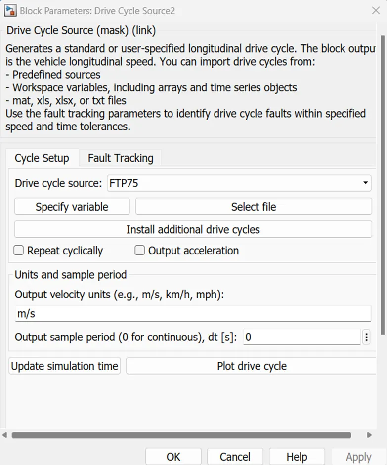
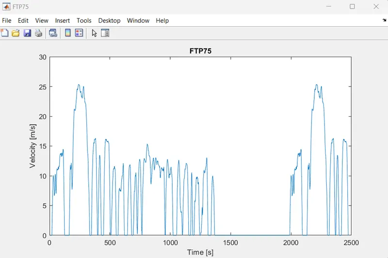
Creates a longitudinal driving cycle that is either predefined or customised. The block output is the longitudinal speed of the vehicle. Drive cycles can be imported from:

established sources

Workspace variables, such as arrays and time series objects in files such as txt, xls, or xlsx

To locate drive cycle problems within the given speed and time limitations, use the fault tracking parameters.

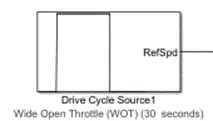
2) Wide Open Throttle (WOT):

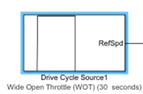
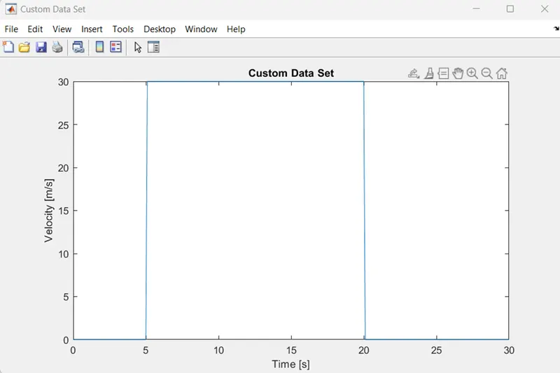
The Wide Open Throttle, or WOT, drive cycle is selected rather than the FTP75 drive cycle using the identical drive cycle source block.

The feedback between the variables in electronic control can be tweaked and used in a variety of ways, even to the point where, in drive-by-wire systems, the operator's input (which is pedal position) is entirely unrelated to throttle position itself. Instead, the computer continuously decides how the two should be correlated as the engine's running condition changes from second to second. During the carburetion period, engines had jets and fuel circuits set up in a certain way to overcome the temporary discrepancies between changes in the throttle position and their influence on how the engine worked (for example, jets to prevent hesitation).

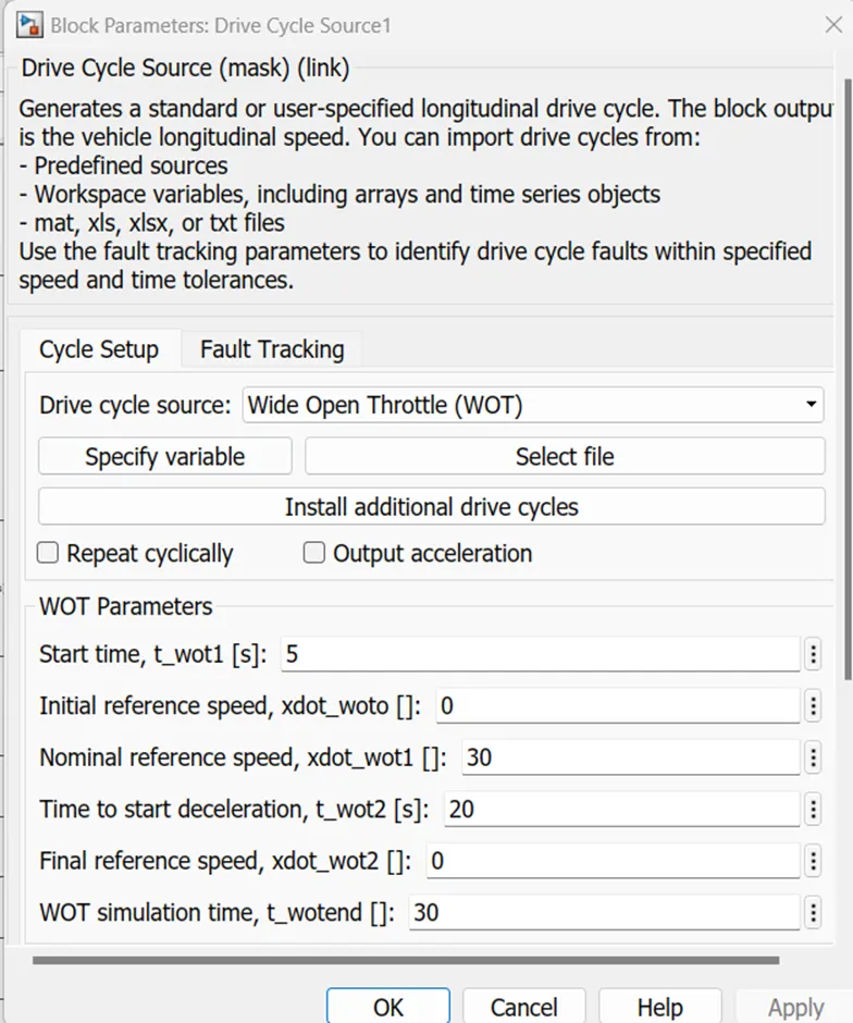
The characteristics show that the vehicle's accelerator or throttle is completely depressed during a 5- to 30-second time range.

(3) 45 Kmph for 100 Kms Drive Cycle:

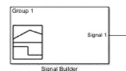
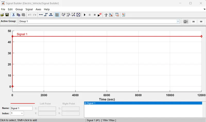
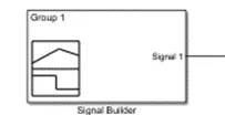
A customised driving cycle is created in accordance with the issue description, in which the car will go about 100 km at a constant speed of 45 km/h. A signal builder block is used to do the same.

Wide Open Throttle is the second driving cycle utilised. Using this specific drive cycle, the car can go 100 kilometres at a continuous 45 kilometres per hour.

The following formula is used to compute this block's parameters:

Here is the time required to go 100 kilometres at a steady 45 kilometres per hour.

Time = Speed / Distance

Time = 100 /(45/3600), where 3600 has been used to convert 45 Kmph to Km/s.

= 8000s

Now, as stated below, are the block parameters for this block.

MATLAB DESIGN:

Inputs and assume data:

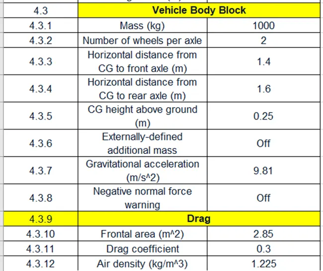
Simulations and testing:

Testing the circuit is the last step after circuit design. Typically, in order to measure the necessary parameters, we must place a scope at any point in the circuit. The scope module like the one in the image below.

Result:

OUTPUT:

1. FTP75:

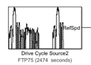
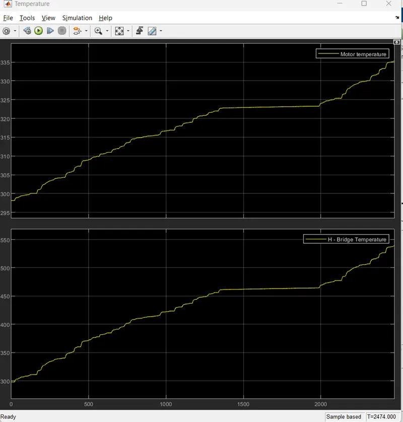
Using the Drive Cycle source FTP75 as a starting point. Every driving cycle has a unique time frame. Therefore, the Drive Cycle source FTP75 has a 2474 second time duration.

1. Travel distance

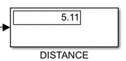
The car has travelled 5.11 kilometers.

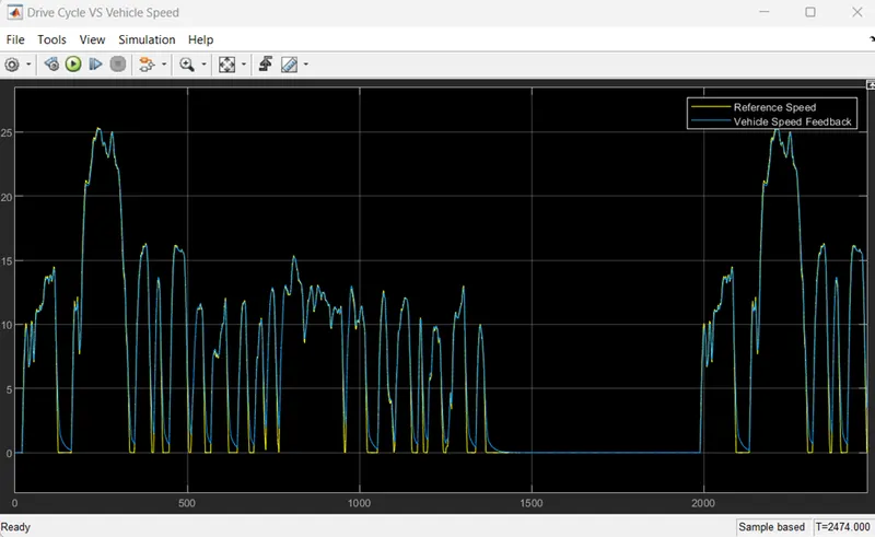
2. The graph of the vehicle's real speed vs its input speed:

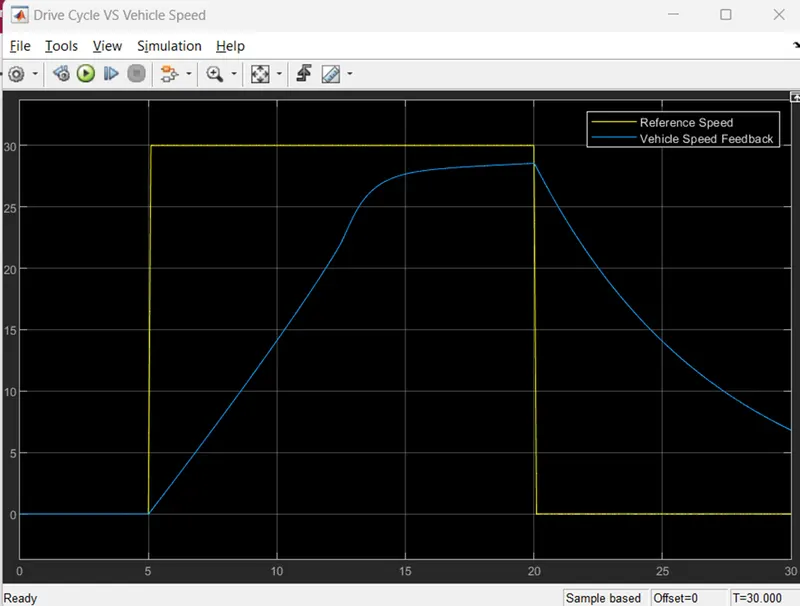
The illustration below demonstrates how closely the real speed of the vehicle follows the reference speed set by the input drive cycle.

Drive Cycle VS Distance:

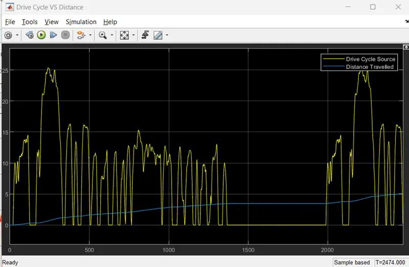
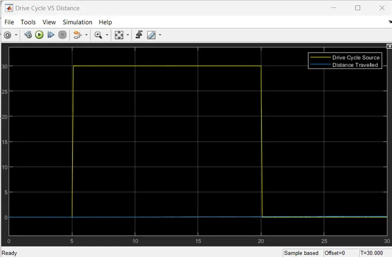
The input vs. output speed comparison graph is shown below. And it was clear that even while the output speed is quite comparable to the input speed, it cannot completely overlap it during acceleration or abrupt deceleration.

3. SOC:

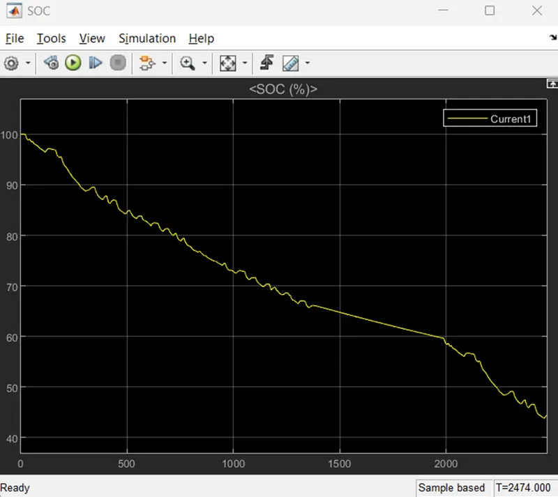
The graph of the SOC percentage.

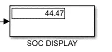
The SOC of vehicle after running for 2474 seconds the battery has changed intermittently from 100% to 79%. During this vehicle has travelled for 5.11 Km. Trend is decreasing but during some time it is increasing. The SOC increases because Regenerative breaking.

The SOC is dropped from 100% to 79%.

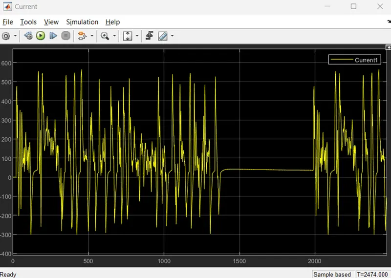
Current:

Energy:

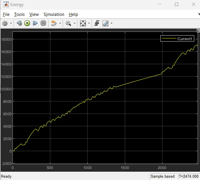
Temperature:

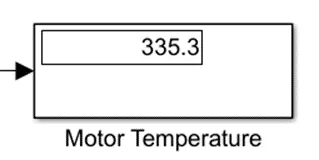
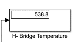
Motor & H- Bridge Temperature:

2. WOT Drive source:

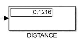
1. Distance travelled:

At the conclusion of the drive cycle, the car has travelled 0.1216 km.

2.The plot for input speed and actual speed of vehicle:

Drive Cycle VS Distance:

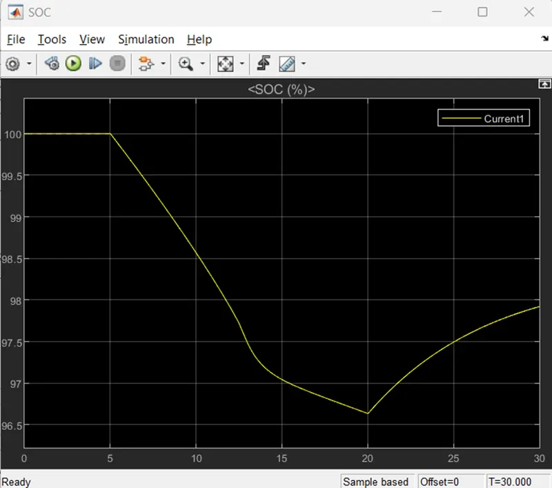
3. SOC

The proportion of SOC on a graph.

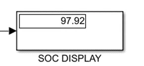
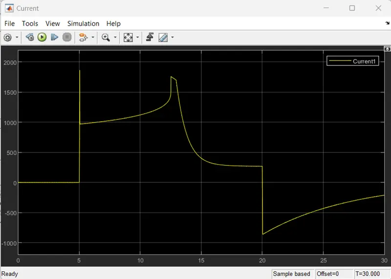
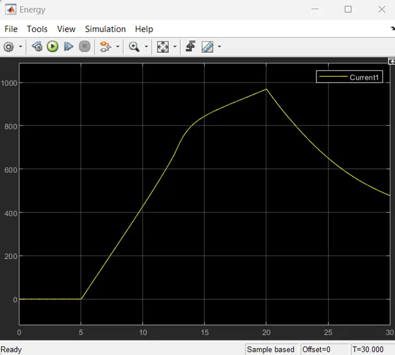
After 2474 seconds of operation, the battery's SOC showed periodic changes from 100% to 99.4%. This car has travelled 0.47 kilometers. While generally declining, there are brief periods when it is rising. Due to Regenerative breaking, SOC rises.

SOC declines from 100% to 97.92%

Current:

Energy:

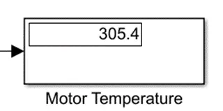
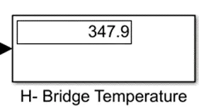
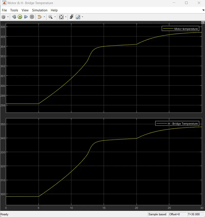
Temperature:

Motor & H- Bridge Temperature:

3) Signal Builder

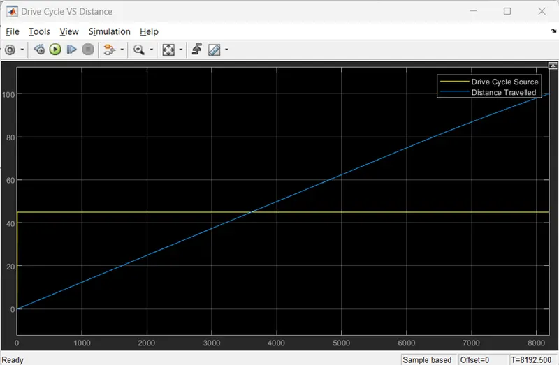
1. Distance Travelled:

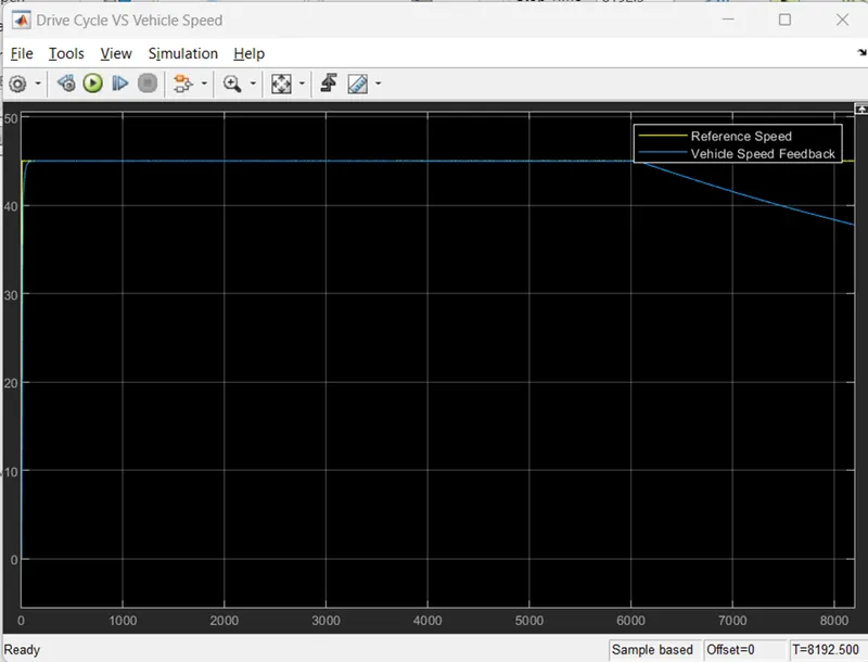
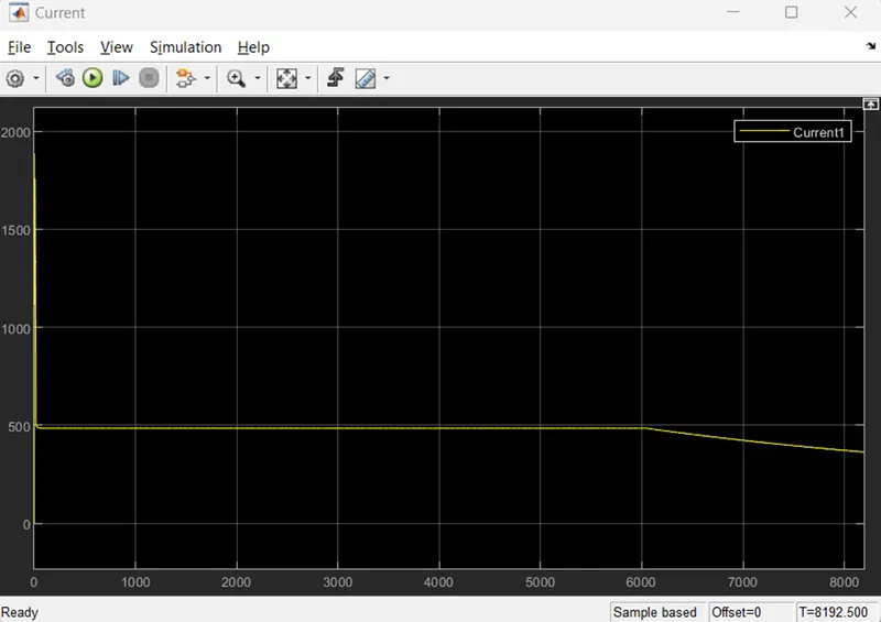
The car has travelled 100 kilometers at 45 Kmph

Here the Simulation time is 8192.5

2. The plot for input speed and actual speed of vehicle:

Drive Cycle VS Distance:

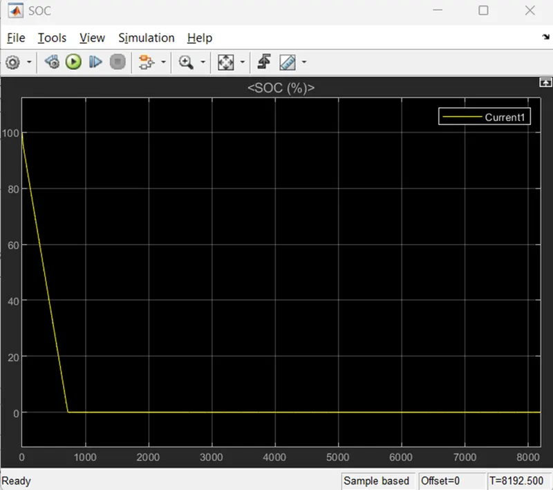
3. SOC:

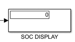
The SOC is dropped from 100% to 0%.

Current:

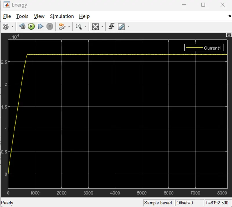
Energy:

Temperature:

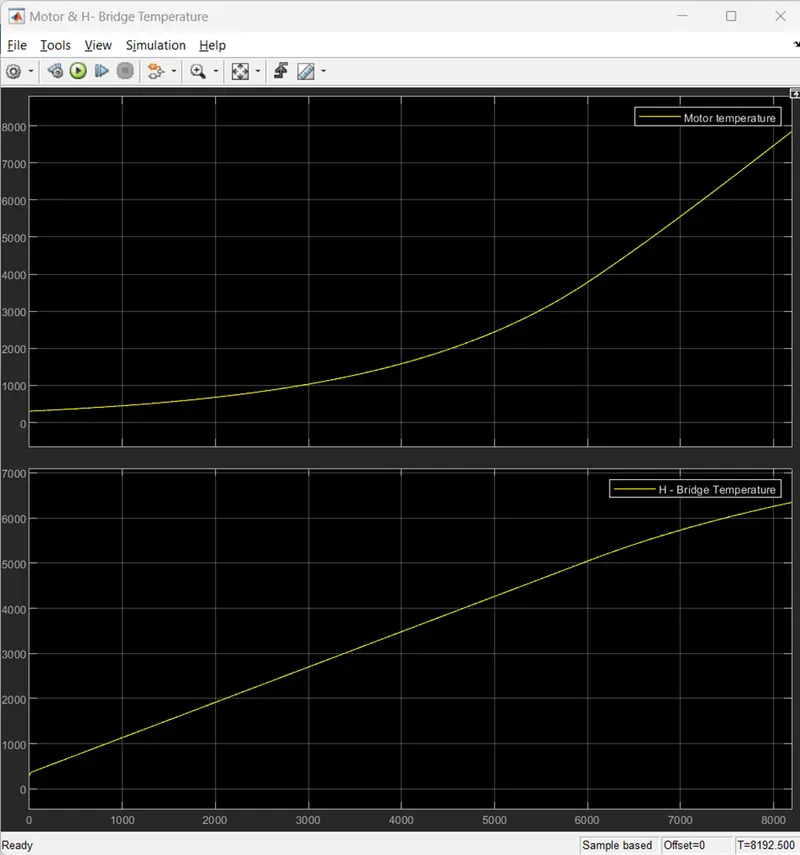
Motor & H- Bridge Temperature:

Conclusion:

• In order to reach a vehicle speed that is close to reference speeds, I have compromised with the temperature of the motor and controller in this case. Due to the lack of a cooling system in the model. The motor temperature in the real-time application is below 100 C.
• In the real-time application, air cooling is used to regulate the temperature of the motor, battery, and controller. As a result, the temperature of these components does not rise as much.
• So, using a Li-ion battery and a PM-brushed DC motor, a MATLAB model of an electric rickshaw (a three-wheeled passenger vehicle) was created.
• determined the differences in the vehicle's energy consumption, SoC%, and motor and controller temperatures for each of the three Reference Drive cycles (i.e.; FTP75, WOT, manually prepared).
• In the future, this battery-powered Rickshaw will be the most widely used form of transportation.