Final Project: Electric Rickshaw modelling

Create a detailed MATLAB model of an electric rickshaw (three-wheel passenger vehicle) as per the details below:

Rear wheels driven by PM brushed type motor

Assume efficiency points of motor controller and motor

Make an excel sheet of all input and assumed data

Results: For any three standard driving cycles show energy consumption, and the temperature rise of the motor and controller for 100 km constant speed driving at 45 kmph.

Aim: To create a Matlab Model of an electric rickshaw using a battery and a permanent magnet brushed motor with Longitudinal driver block and PID block.

Theory:

An electric rickshaw is an Auto that uses electricity as Fuel. To store electricity, batteries are used. These vehicles are becoming popular due less harmful to the environment and these vehicles use electricity as fuel which is cheaper in price.

In this vehicle, electric motors are used which has more than 80% efficiency due to which losses in the system are very less.

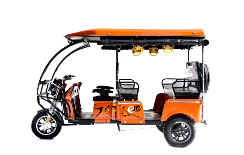
In this project, we are going to design an electric vehicle. Here, we are using a DC motor along with H bridge to move the vehicle. Also, we are going to consider the drive cycle source. In this drive cycle source, there are various types of drive cycle sources are available. We can use 3 different drive cycles and here it should be observed whether the actual velocity is following the drive cycle or not. The blocks used in this model are

1. Vehicle body.
2. Tire.
3. Gear.
4. Motor.
5. H-bridge.
6. PWM Block.
7. Battery.
8. Drive cycle source.

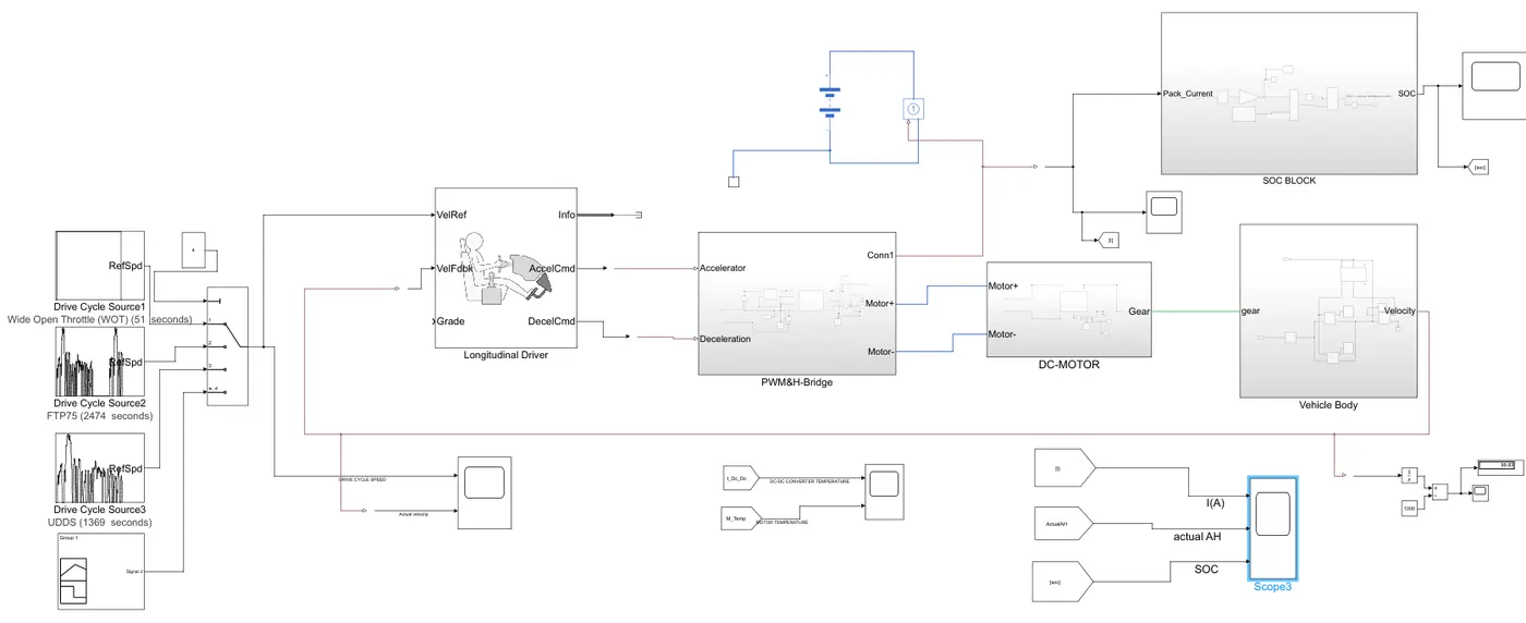
Figure.1. Development of Electric vehicle(Autorickshaw) using MATLAB Simulink.

Here the drive cycles are connected to the longitudinal driver and the acceleration and deceleration is connected to the PWM reference block. The H bridge converter will drive the DC motor. For this motor, the battery is the source.The output of the motor is connected to the gear with a value of 8. The vehicle body block is will gives the actual velocity and in the last block wheels also presented. The SOC block will provides actual AH and maximum AH also. The maximum AH is considered as 50.

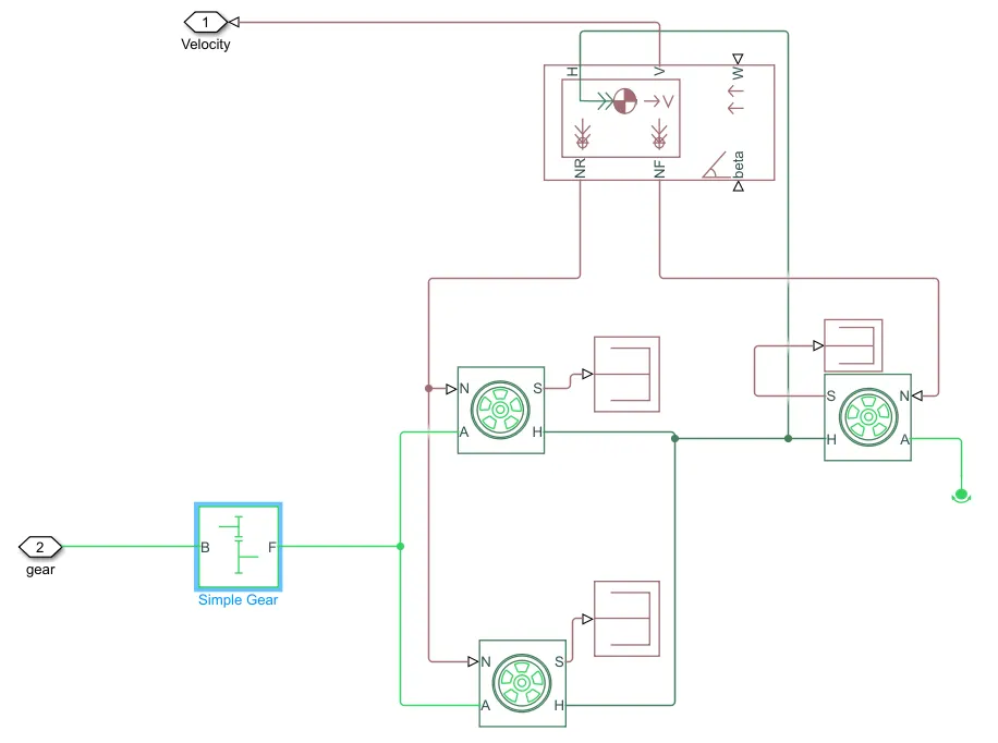
Figure 2. Vehicle along with tires.

The above block consists of vehicle body and four tires. Here NR is connected N terminal of the two tires and NF is connected to another terminals of the single tire. All H terminals of the tire are connected together and the common point are connected to the vehicle body. The ‘S’ terminals of the each tire are terminated here. The ‘W’(wind velocity) terminal is not considered and also the road angle beta is also not considered.

The vehicle body consists of Main, drag, pitch and variables. The corresponding values are shown below figures. Here the mass m is equal to 1200kg and gravitational force is 9.81 and the remaining parameters are kept default values.

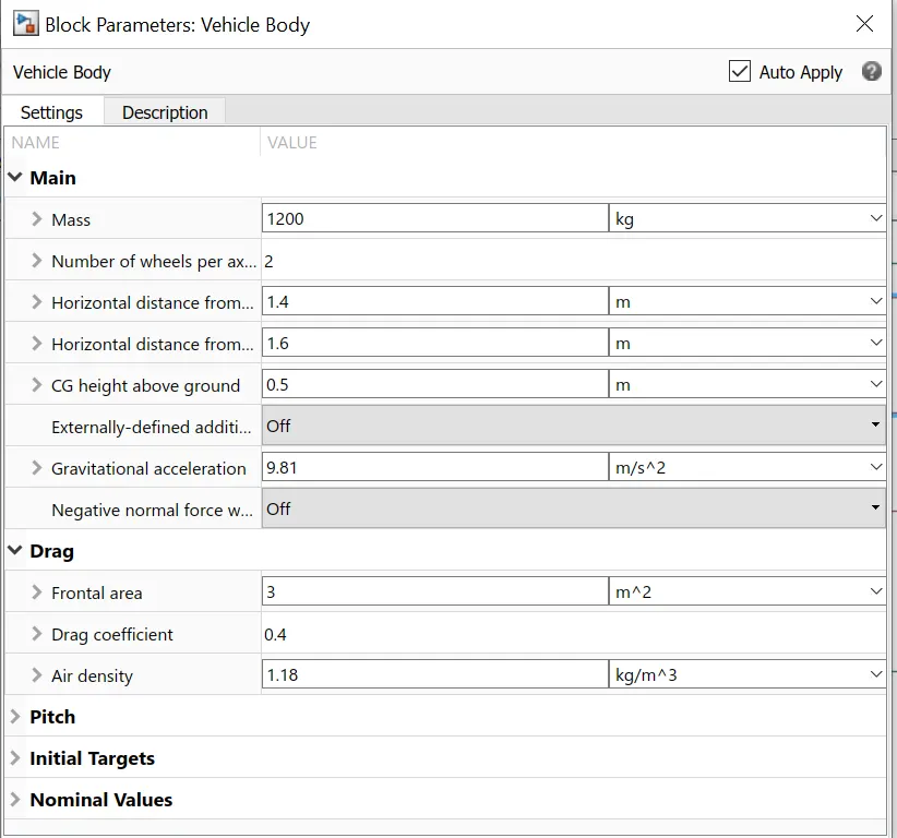
Figure 3. Main and drag Parameters of the vehicle body.

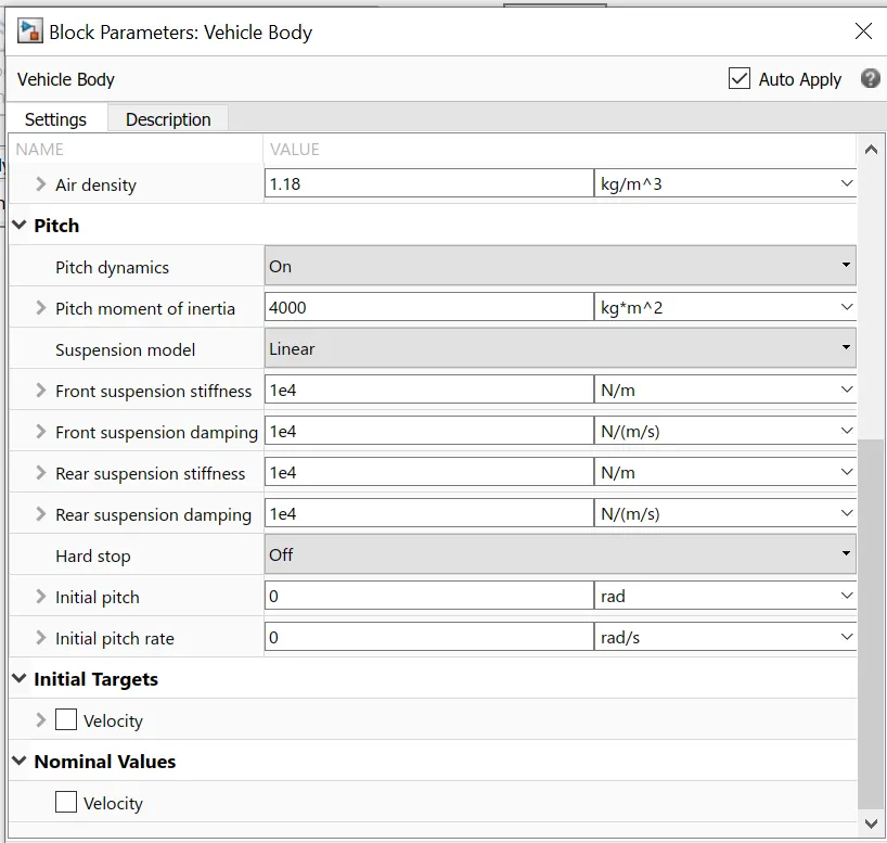
Figure 4. Pitch and other parameters of the vehicle body.

Tyre parameters:

In the tire block parameters block there are 5 parameters

1. Main.
2. Geometry.
3. Dynamics.
4. Rolling resistance.
5. Advanced.

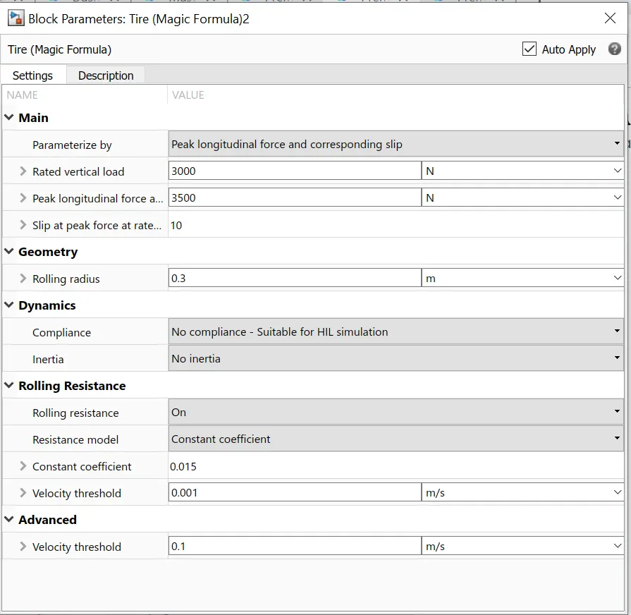
Figure 5. Tyre parameters of the vehicle.

Simple gear parameters:

The gear parameters here I considered as 8. This is based on the actual velocity and reference velocity variation. To get perfect matching I have taken the teeth ratio as 8.

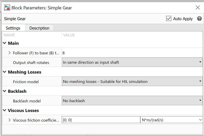
Figure 6. Simple Gear parameters.

Motor Parameters:

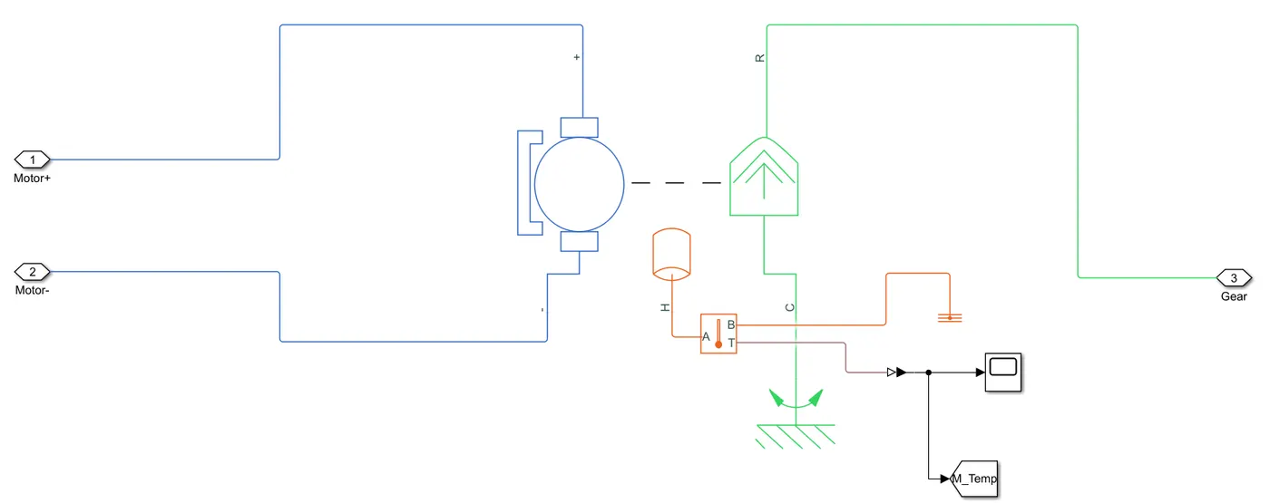
Figure 7. DC MOTOR.

In the DC motor, there are two types of field are available

1. Permanent magnet.
2. Wound.

Here, I have selected a permanent magnet only instead of a wound. Coming to the model parameterization there are different types. The first one is

1. By Equivalent circuit parameters.
2. By rated load and speed.
3. By stalling torque and no-load speed.

Among all these things, I have used rated load and speed. Generally, the voltage for DC motor is 220V. To meet the required power I have chosen as 300V.

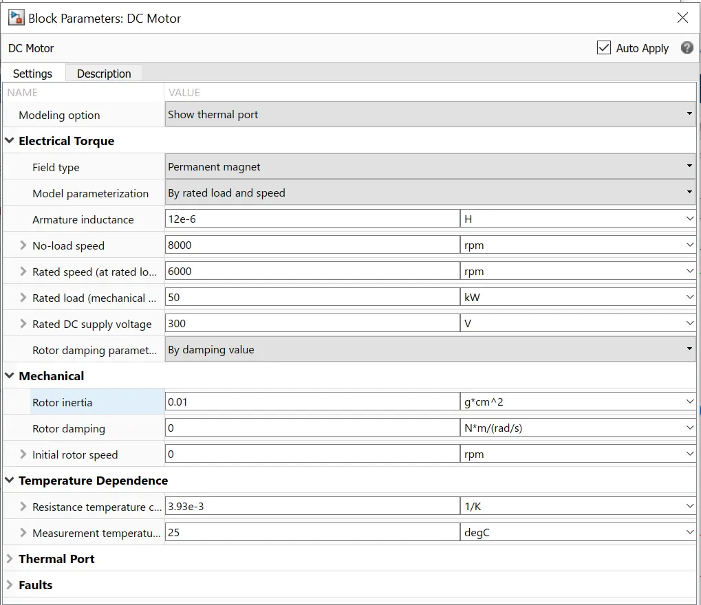
Figure 8. Electrical motor parameters_1.

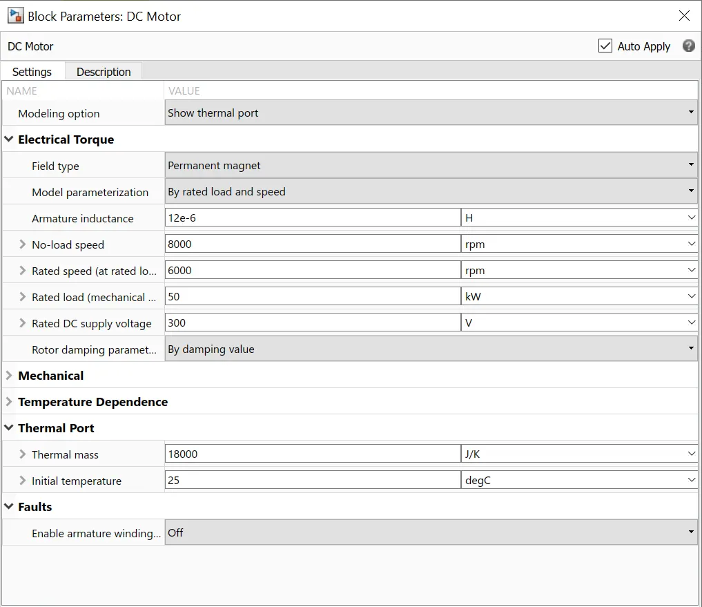
Figure 9. Electrical motor thermal and faults parameters_2.

H Bridge and PWM block:

These blocks are related to power electronics. Here the acceleration port and deceleration ports are connected to dependent voltage sources. The controlled PWM blocks will send PWM signals to the H- bridge. The H-Bridge will give the voltage to the motor. For this H bridge, the voltage is taken from the battery. The PWM frequency here I have considered as 5000Hz and if we increase the PWM frequency the switching losses will increase. Therefore based on the requirement we have to choose the switching frequency. Also, it is observed that the controlled PWM voltage magnitude is 300V. For PWM pulse generation to the power electronics, a voltage of 5V is required. Hence the input scaling block consists of 5V.

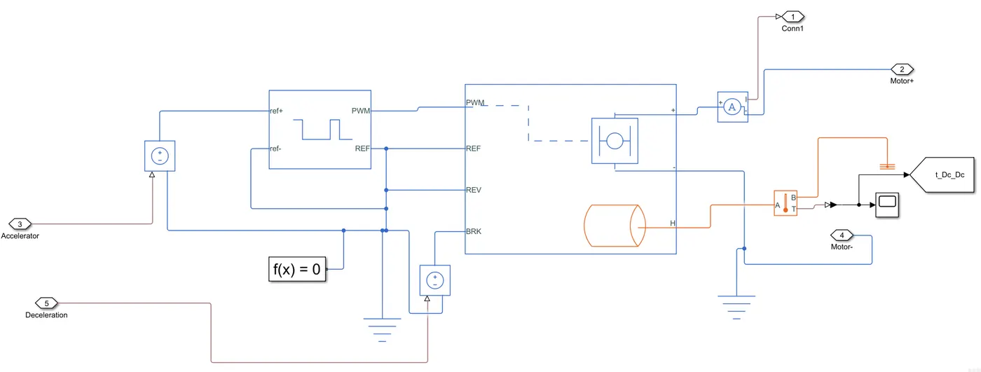
Figure 10. H bridge configaration.

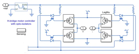
Figure 11. Internal view of H bridge configaration.

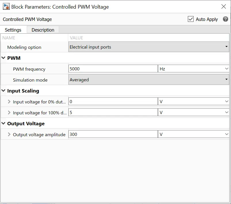
Figure12. Controlled PWM Voltage Parameters.

H bridge: Here in H bridge, I considered the average simulation mode instead of PWM mode. In this mode it will take Ton/T only. Also it is observed that Regenerative braking is enabled. When the drive cycle is in deceleration mode then regenerative braking is obtained.

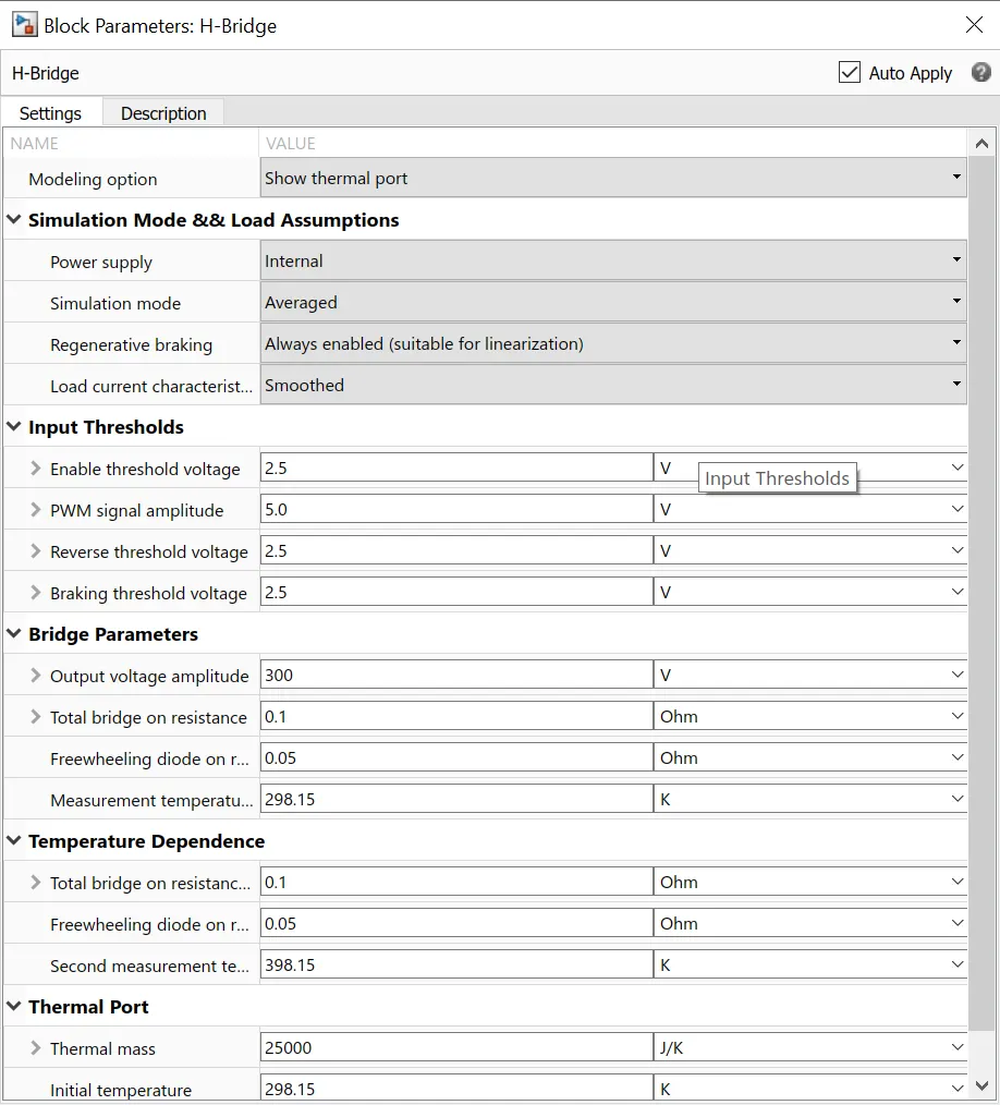
Figure 13 H-Bridge Parameters.

Battery: Here, the main function of the battery is to give the voltage to the H bridge. In this battery already SOC is mentioned. The value of the internal resistance is considered as 0.1ohm. Coming to the charge value the default value is taken i.e 50hr*A.

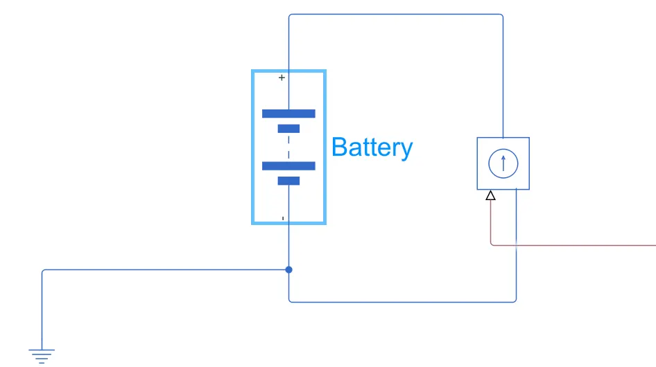
Figure 14 Battery block.

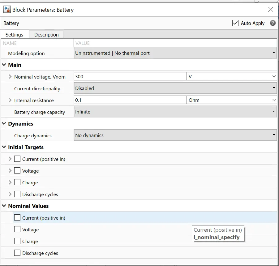
Figure 15. Battery Parameters.

Longitudinal driver: In this block, control type and control parameters are mentioned. The P&I Values can be changed based onactual velocity.

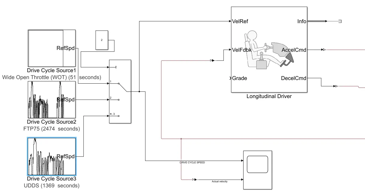
Figure 16. Longitudinal Driver with 3 different drive cycles.

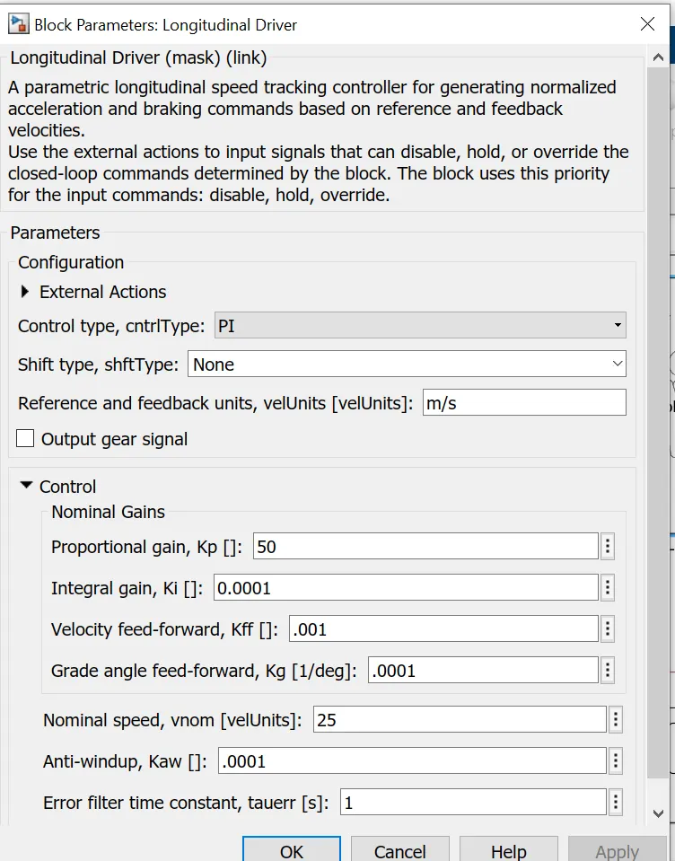
Figure 17. Longitudinal Parameters

Battery SOC:

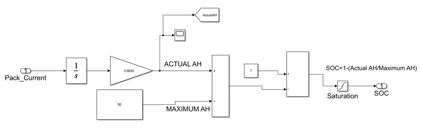
Figure 18. Battery SOC.

To get the charge the current is integrated and the value of the 3600 is to get interms of AH. The maximum AH is considered as 50 and the resultant is subtracted with constant block and produces the value of SOC.

Results: FTP75 Drive Cycle

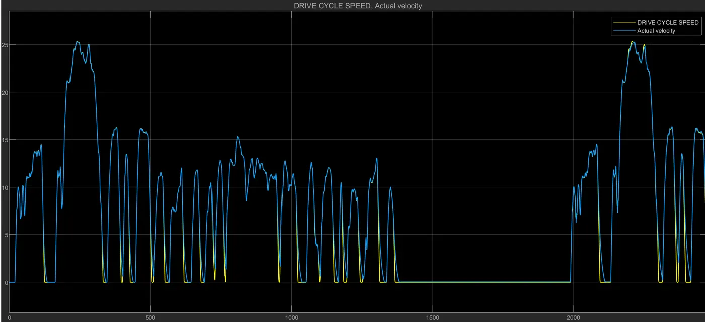
Figure 19. FTP 75 DRIVE CYCLE AND ACTUAL VELCOCITY.

From the above figure, it is clearly understood that velocity(blue) is following the reference drive cycle(yellow). Hence the designed electric vehicle working perfectly.

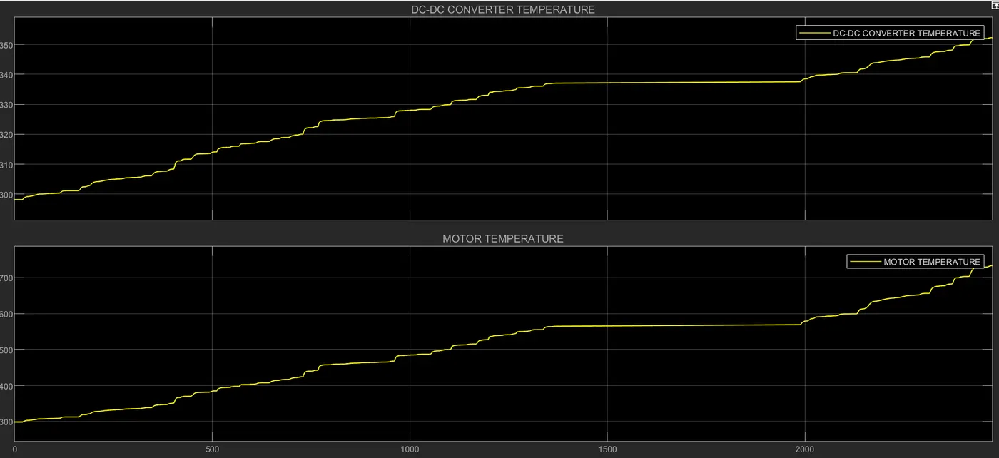
Figure 20. Temperature of DC-DC Converter and Motor in Kelvins.

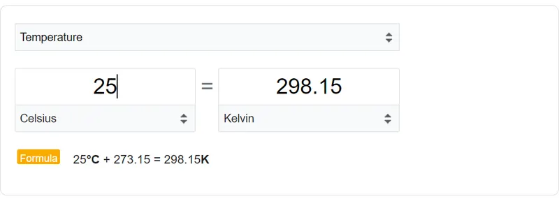
It is observed that in the figure no 9 temperature is 25 degrees celsius and it is converted into kelvins. The same will displayed in the figure no20.

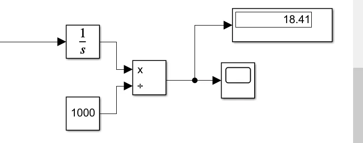
Figure 21. Distance travelled when the vehicle is fed from FTP75 Drive cycle.

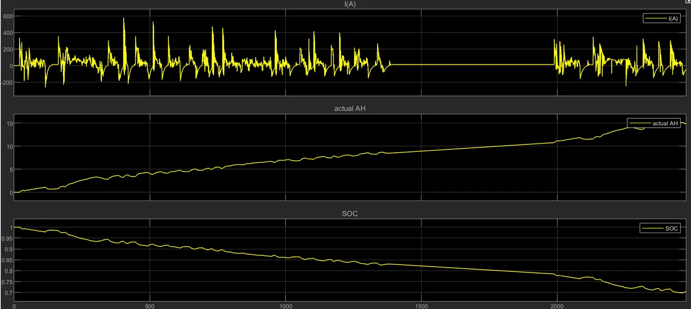
Figure 22. Battery SOC.

UDDS Drive Cycle:

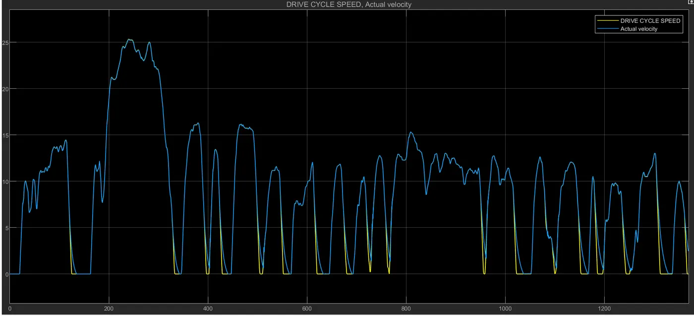
Figure 23. UDDS DRIVE CYCLE AND ACTUAL VELCOCITY.

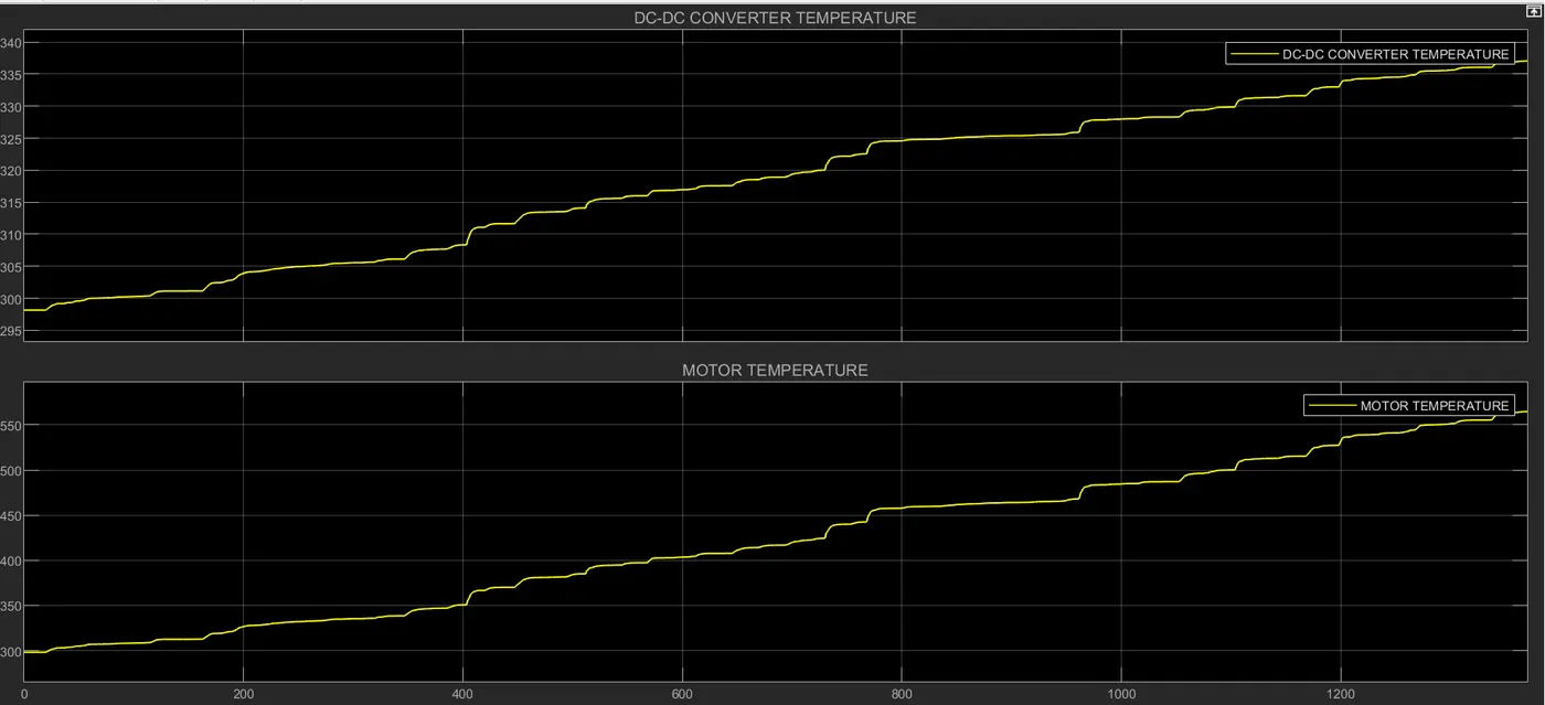
Figure 24. Temperature of DC-DC Converter and Motor in Kelvins.

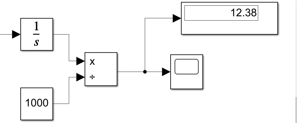
Figure 25. Distance travelled when the vehicle is fed from UDDS Drive cycle.

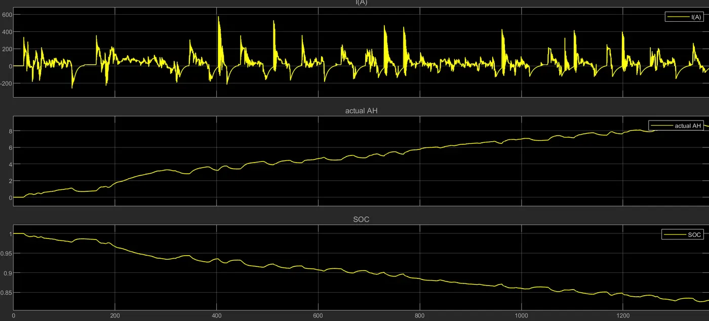
Figure 26. Battery SOC FOR UDDS CYCLE.

WOT CYCLE:

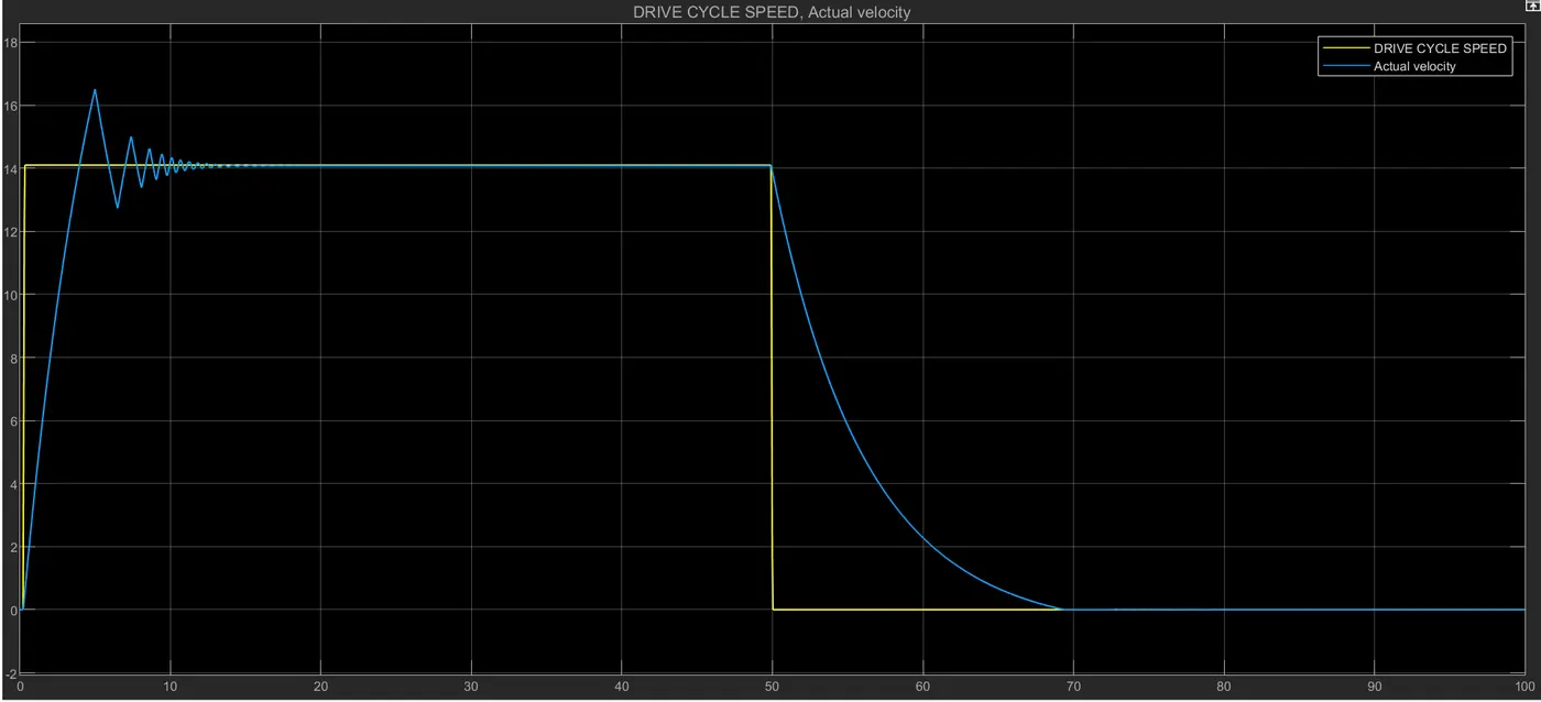
Figure 27. WOT DRIVE CYCLE AND ACTUAL VELCOCITY.

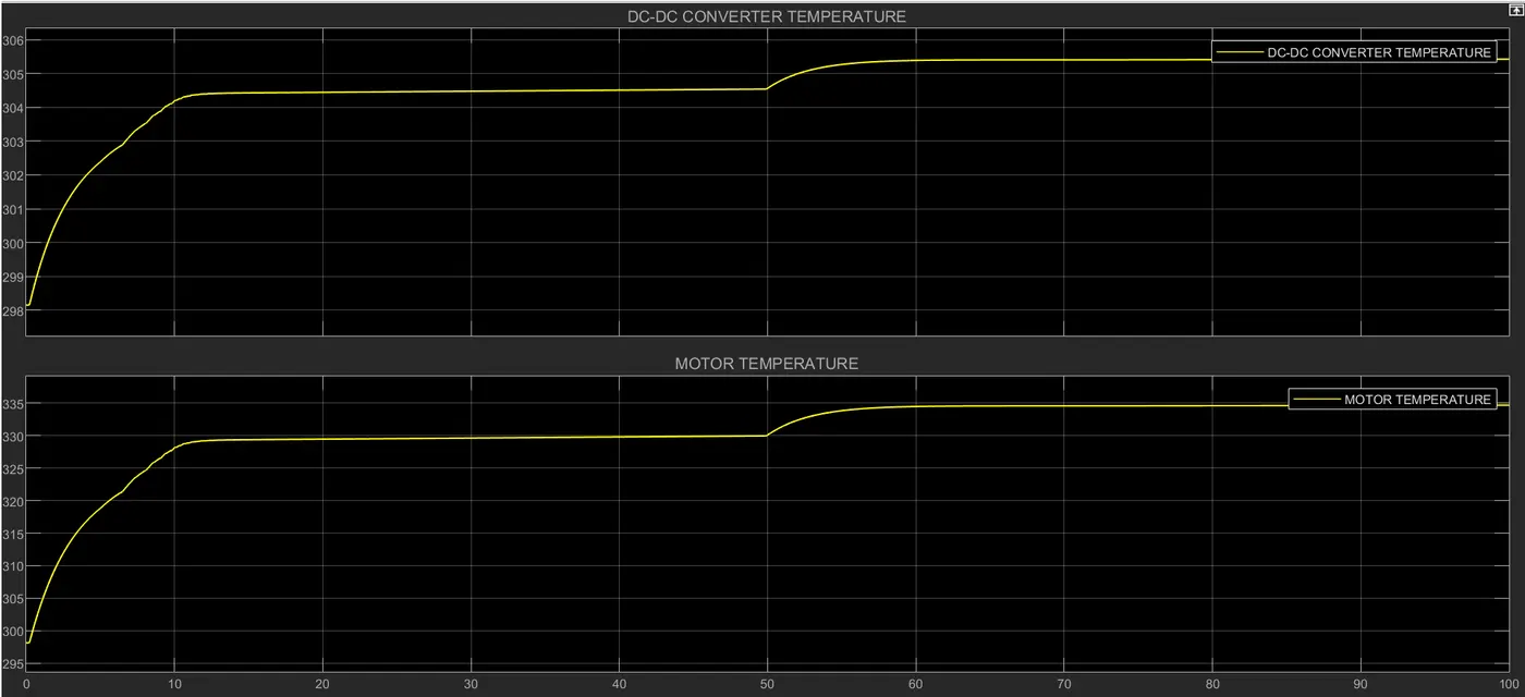
Figure 28. Temperature of DC-DC Converter and Motor in Kelvins.

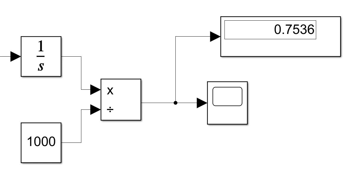
Figure 29. Distance travelled when the vehicle is fed from WOT Drive cycle.

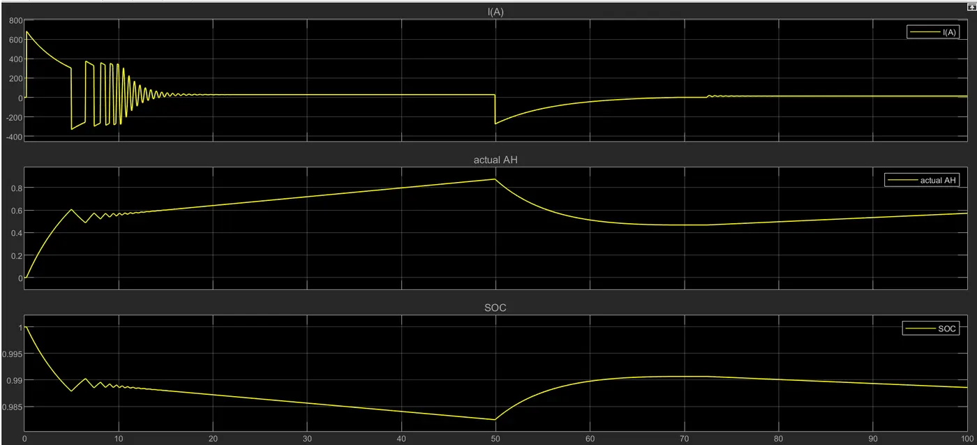
Figure 30. Battery SOC FOR UDDS CYCLE.

4: User defined Drive cycle

As per user the rickshaw need to travel 100Kms with a speed of 45Kmph.

By converting Kmph into m/s ,speed is converterd into 12.5m/s

speed =distance/time

12.5=100000m/time

time=8000secs

Therfore simulation time is 8000secs.

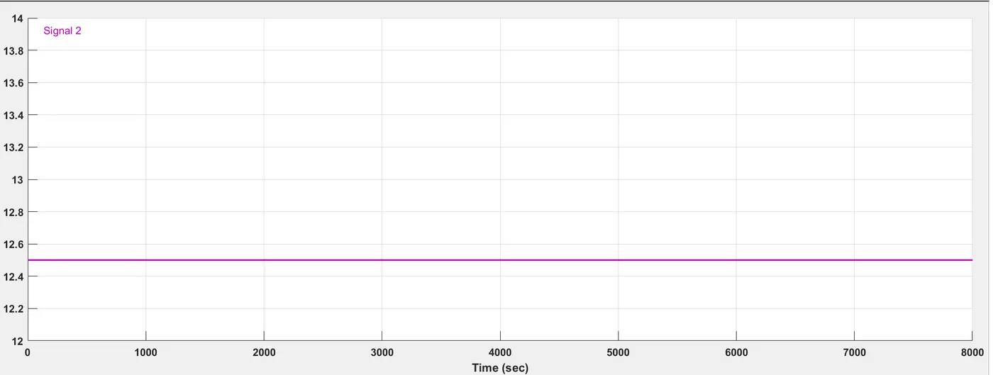
Figure 31. Signal builder for case 4.

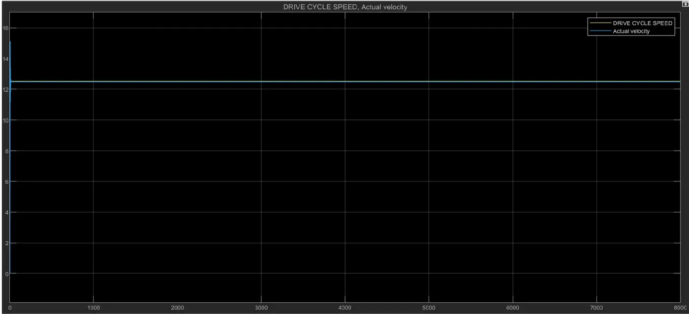
Figure 32. Drive cycle velocity and actual velocity.

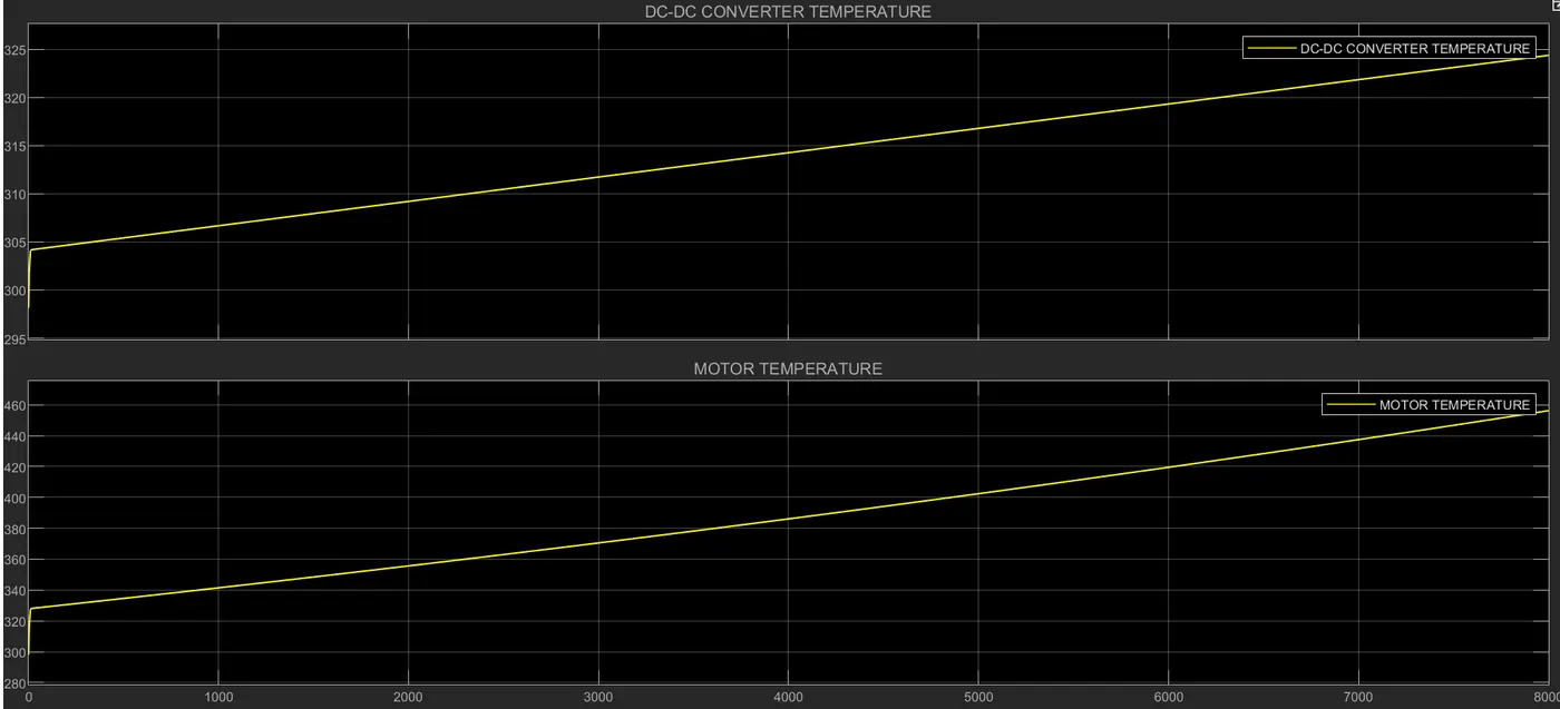
Figure 33. Temperature of DC-DC and Motor.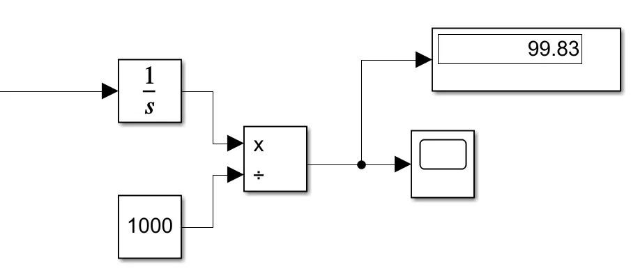

Figure 34. Distance travelled 100km as per the question.

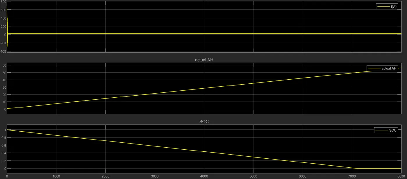
Figure 35. Battery SOC.

Till now we discussed by using longitudinal driver block and now i am replacing the longitudinal block as PID Control as shown in the Figure 36.

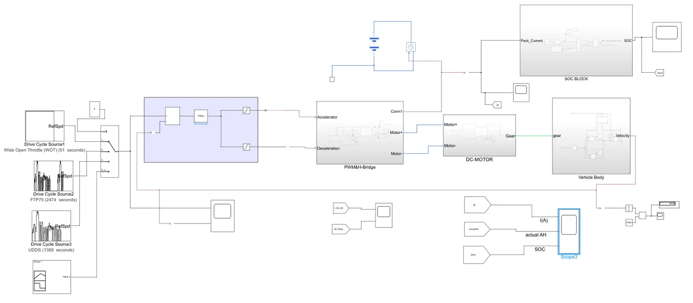
Figure 36. Development of Electric vehicle(Autorickshaw) using MATLAB Simulink and PID Controller.

WOT CYCLE:

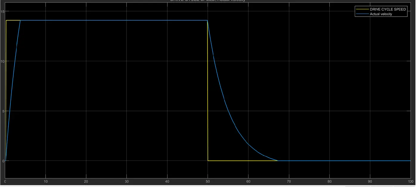
Figure 37. WOT Drive cycle and Actualy velocity using PID Controller.

It is observed that from the figure 27 a small peak over shoot occurs when we are using a longitudinal driver block but whereas from figure 37 it is observed that there is no peak overshoot (this is when we are using PID only)

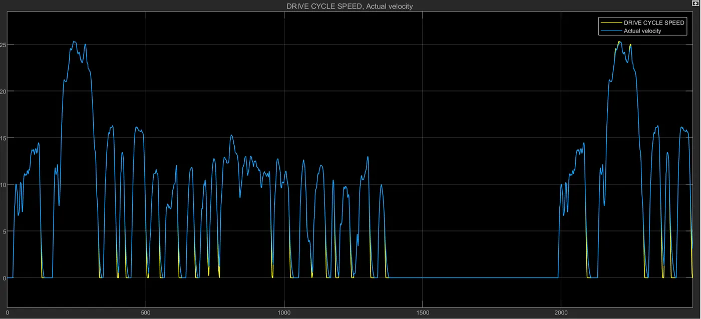
Figure 38. FTP75 Drive cycle and Actualy velocity using PID Controller.

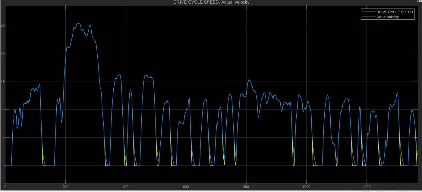
Figure 39. UDDS Drive cycle and Actualy velocity using PID Controller.

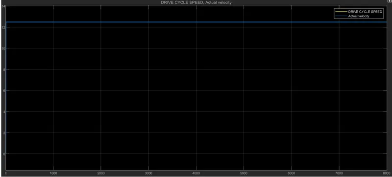
Figure 40. Constant Drive cycle and Actualy velocity using PID Controller.

Conclusion:

1. The electric rickshaw is developed using matlab software with longitudinal driver and PID Controller.

2. Both files are simulated and results have been presented for both the cases. The results for both cases are almost similar.

3. The 100km distance with 45km speed case also solved and image of the distance has been attached.

4. FTP75, WOT and UDDS drive cycles are also implemented and results have been presented for temperature and distance also.

5. Assumed data also explained clearly along with the images AND Excel sheet of sample data is attached.

6. Two MATLAB FILES(Longitudinal driver and PID Control) have been attached for proper verification.