Project 1: ELECTRIC RICKSHAW (3-WHEELER) MODELLING

• Project 1: Modelling of an Electric Rickshaw (3 Wheeler Passenger Vehicle)

I. OBJECTIVES

• To create a detailed MATLAB model of an electric rickshaw (three-wheel passenger vehicle) as per the details below:

1. Rear wheels driven by PM brushed type motor
2. Assume efficiency points of motor controller and motor
3. Make an excel sheet of all input and assumed data
4. Results: For any three standard driving cycles show energy consumption and the temperature rise of the motor and controller.

II. BRIEF INTRODUCTION

• About E-Rickshaws (Electric 3-wheelers)
  

  Urban development in India has resulted in a rise in the number of cities from 5,161 (2001) to 7,935 (2011) 1, along with an indicative concentration of population in cities and existing urban agglomerations. As per 2011 data, 53 cities had populations greater than a million and about 377 million people were residing in towns 2. With this, a notable rise in demand for vehicles was also observed for inter-city or intra-city mobility of goods and passengers. A considerable rise in the number of registered vehicles (25.3 times against the population growth of 1.77 times between 1981 and 2011) was also observed, further indicating the need for viable passenger mobility solutions. Million plus cities in India have observed a similar trend of increase in vehicular population (e.g., Delhi witnessed growth from 3,635 vehicles in 2001 to 7,228 in 2011 3) with a simultaneous rise in issues related to vehicular emissions. Conventional fuel-powered vehicles, currently available as mobility modes largely contribute to pollution and emissions, leading to poor air quality, health problems, and various other issues. The need to combat these issues has been realized by cities and alternative mobility options are being explored. Electric vehicles (EVs) are increasingly being considered the most logical option for achieving the aim of combating local air pollution through alternative-powered vehicles. In recent times EV technology has matured and is being promoted in line with zero tailpipe emissions. These are soon becoming a smart alternative for conventional fuel vehicles in India. The strongest push to shift towards electric modes comes from the national government, through the promotion of various programs, schemes, and policy support. Since 2011, the national government has been making efforts to introduce a transition from conventional vehicles to electric vehicles. Ministry of Heavy Industries (MoHI) launched National Electric Mobility Mission Plan (NEMMP) in 2013. Later in 2015, the Department of Heavy Industry (DHI) introduced the FAME I (Faster Adoption and Manufacturing of Hybrid & Electric Vehicles) scheme, followed by FAME II (in 2019). In addition, India’s vision of Intended Nationally Determined Contribution (INDC) specifies a decarbonization target of 33- 35% concerning GDP between 2005–2030, 4 supported by the Draft National Energy Policy (June 2017). In 2018, GoI announced at the MOVE global summit that discussions to introduce ‘E-Cess’ on fuel-powered vehicles are ongoing. Recently in February 2019, the Ministry of Power issued guidelines and standards for setting up charging infrastructure for electric vehicles as an amendment to the Model Building Byelaws 2016, supporting long-term India’s vision of implementing electric mobility 6. Along with these national government efforts, notable initiatives like Smart city mission (2015) and Atal Mission for Rejuvenation and Urban Transformation (AMRUT 2015) laid respective emphasis on multi-modal options for last-mile connectivity along with the development of supporting infrastructure, targeting mass-scale EV integration in future. Initiatives at the national level further triggered states to initiate the development of a prominent policy landscape around EV adoption. States including Telangana, Karnataka, Delhi, Kerala, Maharashtra, Uttar Pradesh, and Uttarakhand have announced EV-focused policies. Though the EV sector includes modes of public transport (PT), private transport (PV), and last-mile connectivity with fast-developing policies/ initiatives but still an example of an often ignored mode for urban mobility is the modest e-rickshaw. A recent report published by Deloitte stated that e-rickshaws can be ‘low hanging fruits’ in EV adoption due to low life cycle cost, 7 thus a better understanding of this mode may result in the effective deployment of modal combination. E-rickshaws are zero tailpipe emission modal options used as first/last mile connectivity in cities. These 3-wheeled electric-powered vehicles are usually expected to complete the value chain of public transport service gaps, for commuters. These have net power of less than 4000 W, a speed restriction of 25kmph, and a seating capacity for four passengers along with the driver. E-rickshaws are welcomed by commuters and operators due to their characteristics of being demand-responsive, comfortable, affordable, flexible, and convenient. However, with the uncontrolled rise in the number of e-rickshaws, their regulation has become a challenge for authorities. 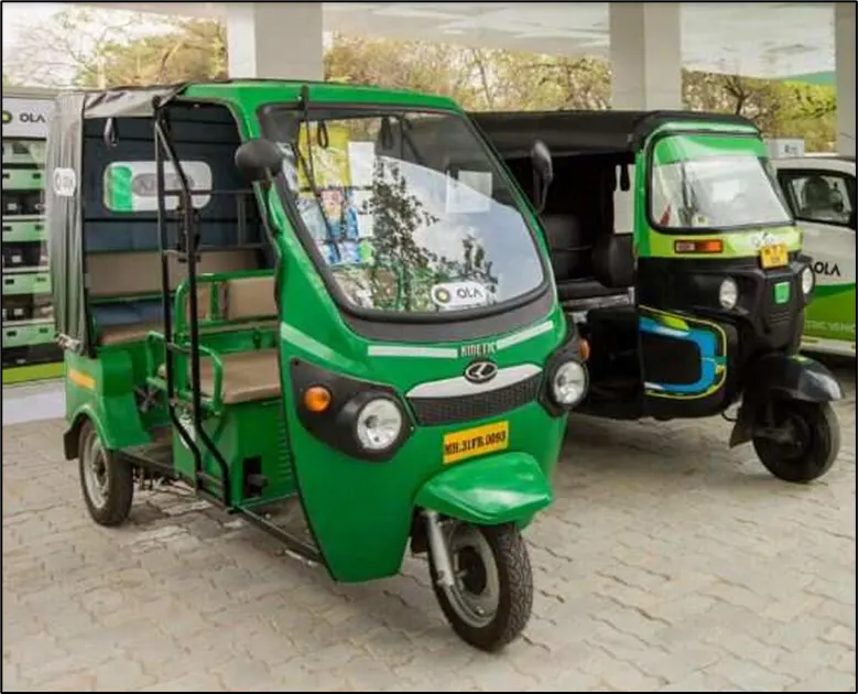Fig.1. Two E Rickshaws at an Auto event

• About Electric Vehicle Powertrain

  The powertrain of a Battery Electric Vehicle (BEV) consists of an electric drive system with a battery serving as an energy buffer. Often there is only one electric machine (DC Motor), connected to the wheel shaft via a gearbox and a differential. However, some applications may utilize several electric machines, e.g., hub wheel motors. The energy is stored chemically in a battery, which is electrically connected to the machine via a DC/AC power electronic converter accompanied by a control system. The control system controls the frequency and magnitude of the three-phase voltage applied to the electric machine, which depends on the driver’s present request, which is communicated via the acceleration and/or brake pedal. In the case of vehicle applications, it is usually desirable to keep the physical volume of the electric machine down. This can be done by designing it for higher speed levels. A reasonable compromise is a maximum speed between 12 000 to 16 000 rpm since it serves as a good compromise between volume and performance. Still, during normal on-road driving the speed range of a vehicle may vary between zero to about 130 km/h or even higher at times. This means that the wheels will spin up to around 1200 rpm or higher. Therefore, a reduction gear ratio toward the wheels is inherently needed. Additionally, to give the left and right traction wheels a chance to spin at slightly different speeds during turning, there is also a need for a differential to be connected between the wheels. Sometimes the differential also includes a final gear ratio. A typical BEV drive system is depicted in Figure 2. 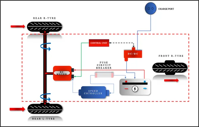Fig.2. Typical schematic of a 3-wheeler EV

III. CASE STUDY

• Simulink Model - E Rickshaw (Electric 3-Wheeler Vehicle) Model

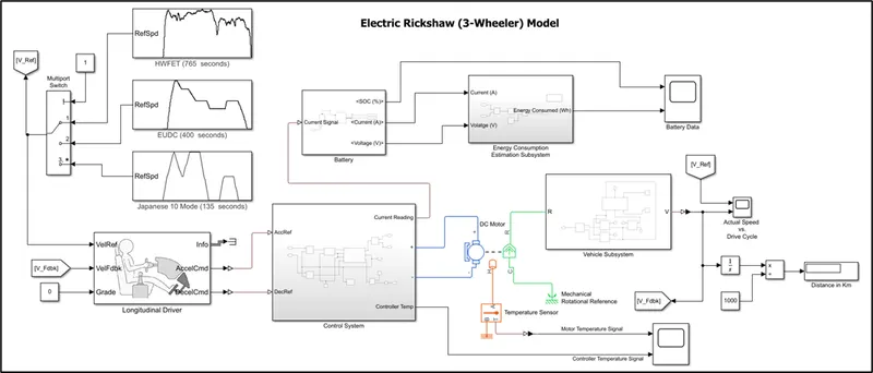
  Fig.3. Simulink Model for our EV

1. Model Parameters:-
   
   For this project, we have considered the vehicle model parameters of the Mahindra Electric Treo-SFT.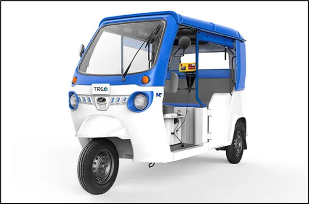

   Fig.4. Image of the Treo E Rickshaw

   
   

   Vehicle Specifications:

   `"Kerb Weight"`	`=`	`"377 Kg"`
   `"Payload"`	`=`	`"123 Kg"`
   `"Coefficient of Rolling Resistance," μ_( r r)`	`=`	`"0.015"`
   `"Frontal Area"`	`=`	`"2.3625" m^2`
   `"Coefficient of Drag," C_(D)`	`=`	`"0.24"`
   `"Acceleration Time (0 to 55 kmph)"`	`=`	`"6 sec"`
   `"Gradeability"`	`=`	`"12.7"^circ`

   
   Vehicle Performance Calculations:
   We use our excel calculator for the propulsion power requirement calculations.
   
   

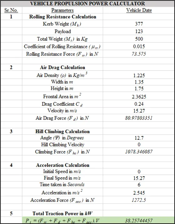
   Fig.5. Excel Calculator

   
   From the above calculations, it is clear that the maximum propulsion power required is 38.25 kW. If we calculate the Torque value based on this, we will get 381.95 Nm at the wheel (assuming a tire radius of 0.1524 m). Hence, we consider a higher value to overcome traction issues during operation and consider a value of 45 kW.
   
   DC Motor Calculations:
   Since we know that the transmission in the Treo-SFT is a Direct drive, an assumption of maximum transmission efficiency of 98% is made and we can calculate the highest output torque at the output shaft;
   `"Input Torque from Motor" = "Output Shaft Torque"/"Transmission Efficiency" = 381.95/0.98`
   `:. "Output Torque" = 389.7Nm`
   Hence, the motor is more than capable of handling these torque conditions.
   Based on this we can calculate the full load speed;
   `"Motor Speed " = ("Power"xx60) / (2pixx "Torque") = (45000 xx60)/(2pixx389.7) = 1125 RPM`
   
   Tire Calculations:
   From the specifications, the Treo-SFT uses tires with the code - 10 R 20.
   From the company website, the final rolling radius is evaluated to be 0.1524 m. We will assume the Load Index to be 89 (1279 lb).
   
2. System-Level Configurations:-
   
   [A] Drive Cycle Source:
   

   The Drive Cycle Source block generates a standard or user-specified longitudinal drive cycle. The block output is the specified vehicle longitudinal speed, which you can use to:

   • Predict the engine torque and fuel consumption that a vehicle requires to achieve desired speed and acceleration for a given gear shift reference.

   • Produce realistic velocity and shift references for closed-loop acceleration and braking commands for vehicle control and plant models.

   • Study, tune, and optimize vehicle control, system performance, and system robustness over multiple drive cycles.

   For our study, we have chosen two drive cycles as follows;
   
   

   I. HWFET (765 seconds)

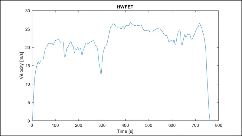
   Fig.6. HWFET Drive cycle

   II. EUDC (400 seconds)

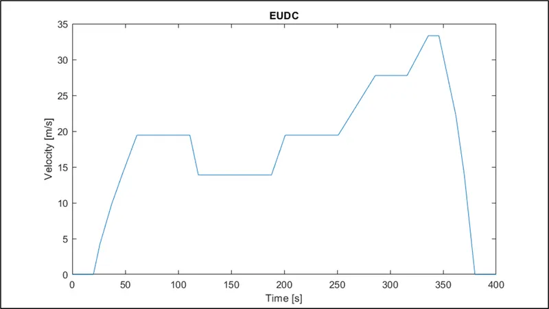
   Fig.7. EUDC Class 2 Drive cycle

   III. Japanese 10 Mode (135 seconds)

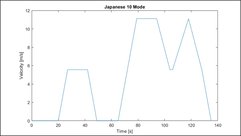
   Fig.8. Japanese 10 Mode Drive cycle

   
   These drive cycles can be switched whenever necessary. For this purpose, a Multiport Switch block is used which changes the input of the drive cycles.
   
   [B] Longitudinal Driver Block:
   The Longitudinal Driver block implements a longitudinal speed-tracking controller. Based on reference and feedback velocities, the block generates normalized acceleration and braking commands that can vary from 0 through 1. You can use the block to model the dynamic response of a driver or to generate the commands necessary to track a longitudinal drive cycle. We use the default values for the PI control. Since there is no automated way of tuning the PI controller in this block, we rely on the default parameters.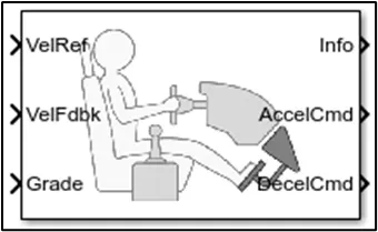

   Fig.9. Longitudinal Driver Block

   
   I. VelRef - Reference Vehicle velocity that is directly connected with the Drive cycle output.
   II. VelFdbk - Longitudinal vehicle velocity in the vehicle-fixed frame, or, feedback velocity from the vehicle.
   III. Grade — Road grade angle (constant input in our case)
   IV. AccelCmd — Commanded vehicle acceleration
   V. DecelCmd — Commanded vehicle deceleration
   
   [C] Control Subsystem: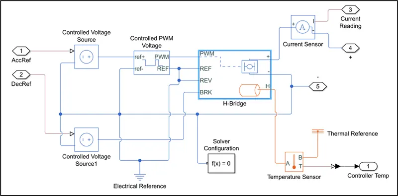

   Fig.10. Control Subsystem

   
   - Controlled Voltage Source Blocks
   The Controlled Voltage Source block converts a Simulink input signal into an equivalent voltage source. The generated voltage is driven by the input signal of the block. We use two of these blocks to provide output signals as directed by the output from the Longitudinal Driver block for Acceleration and Deceleration commands respectively.
   
   - Controlled PWM Voltage Block
   The Controlled PWM Voltage block represents a pulse-width modulated (PWM) voltage source.
   Electrical input ports — The block calculates the duty cycle based on the reference voltage across its ref+ and ref- ports. This modeling variant is the default.
   PS input — Specify the duty cycle value directly by using an input physical signal port.

   For the Electrical input ports variant of the block, the demanded duty cycle is `(V_(ref) - V_(min))/(V_(max) - V_(min)) *100 %` where: Vref is the reference voltage across the ref+ and ref- ports. Vmin is the minimum reference voltage. Vmax is the maximum reference voltage. The value of the Output voltage amplitude parameter determines the amplitude of the output voltage. At zero, the pulse is initialized as high, unless the Pulse delay time parameter is greater than zero, or the demanded duty cycle is zero. For a 100% duty cycle, the input voltage is set to 0.01V for accurate mapping of the output signals from the driver block.

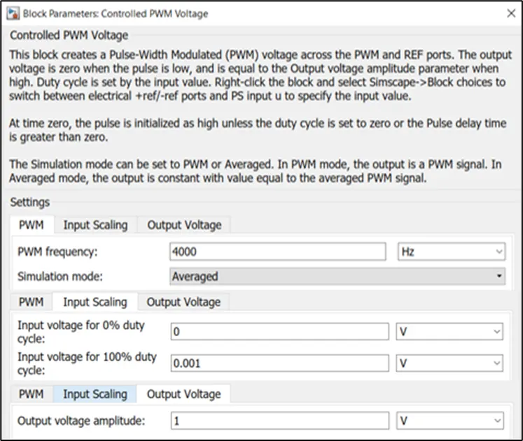
   Fig.11. Controlled PWM Block Configuration

   
   - H-Bridge Block
   The H-Bridge block represents an H-bridge motor driver. The block can be driven by the Controlled PWM Voltage block in PWM or Averaged mode. In PWM mode, the motor is powered if the PWM port voltage is above the Enable threshold voltage. In Averaged mode, the PWM port voltage divided by the PWM signal amplitude parameter defines the ratio of the on-time to the PWM period. Using this ratio and assumptions about the load, the block applies an average voltage to the load that achieves the correct average load current. The Simulation mode parameter value must be the same for the Controlled PWM Voltage and H-Bridge blocks.
   
   If the REV port voltage is greater than the Reverse threshold voltage, then the output voltage polarity is reversed. If the BRK port voltage is greater than the Braking threshold voltage, then the output terminals are short-circuited via one bridge arm in series with the parallel combination of a second bridge arm and a freewheeling diode. Voltages at ports PWM, REV, and BRK are defined relative to the REF port.
   + — Positive Load Connection port
   - — Negative load connection port
   PWM — Pulse-width modulated signal (associated with the pulse-width modulated signal. The voltage is defined relative to the REF port)
   REF — Reference (associated with the floating zero volt reference)
   REV — REV (associated with the voltage that controls when to reverse the polarity of the H-Bridge block output. The voltage is defined relative to the REF port)
   BRK — BRK (associated with the voltage that controls when to short circuit the H-Bridge block output. The voltage is defined relative to the REF port)
   H — Thermal port (The heat generated by the bridge on-resistance and freewheeling diodes is added to the thermal port. The thermal port has an associated thermal mass and initial temperature that you can set from the Thermal Port parameters)
   
   The output signals from the Driver block are mapped in mV. This means that the change in acceleration or deceleration is measured at smaller magnitudes of voltage. Hence, the input threshold voltages for the H-Bridge shall be set to 0.01 V for accurate control of the DC motor.
   
   To attain the thermal parameters of the H-block, we use the "show thermal port" option by right-clicking on the block itself. Figure 12 shows the block parameters.
   

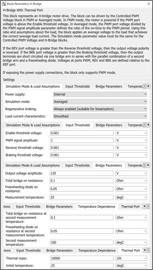
   Fig.12. H-Bridge Block Configuration

   
   - Current Sensor Block
   

   The block represents an ideal current sensor, that is, a device that converts current measured in any electrical branch into a physical signal proportional to the current.

   Connections + and - are conserving electrical ports through which the sensor is inserted into the circuit. The connection 'I' is a physical signal port that outputs the current value.
   The output signal from this block will be used to measure the SoC of the battery.
   
   
   - Temperature Sensor Block
   
   The Temperature Sensor block represents an ideal temperature sensor, that is, a device that determines the temperature differential measured between two points without drawing any heat.

   Connections A and B are thermal conserving ports that connect to the two points where the temperature is being monitored. Port T is a physical signal port that outputs the temperature differential value.

   The block positive direction is from port A to port B. The measured temperature is determined as T = T_A – T_B.

   
   [D] DC Motor Block:
   
   

   
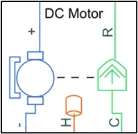
   This block represents the electrical and torque characteristics of a DC motor.

   The block assumes that no electromagnetic energy is lost, and hence the back-emf and torque constants have the same numerical value when in SI units. Motor parameters can either be specified directly or derived from the no-load speed and stall torque. If no information is available on armature inductance, this parameter can be set to some small non-zero value.
   + — Positive terminal
   - — Negative terminal
   C — Motor case
   R — Motor rotor
   H — Thermal port
   
   We can configure this block with the values we had previously calculated in the parameters. According to the parameters, the Rated Speed is given as 1125 RPM, Rated Load is set to 45 kW, and the DC supply voltage is kept at 120V.
   Similar to the H-Bridge, the thermal port is enabled for the motor block. Here, the thermal port is used to simulate the effects of copper resistance losses that convert electrical power to heat.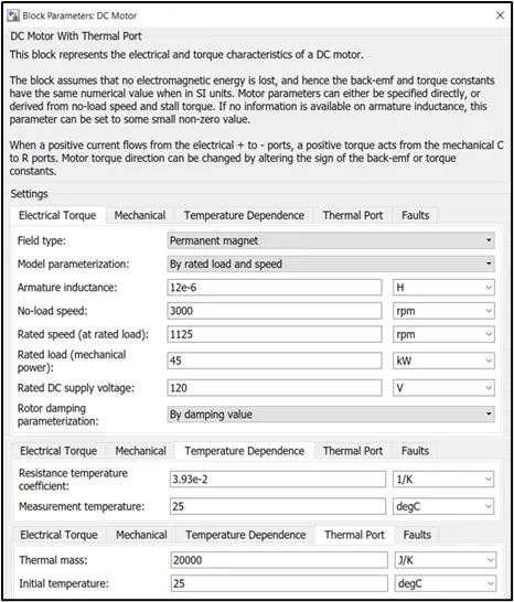

   Fig.13. DC Motor Block Configuration

   
   [E] Vehicle Subsystem: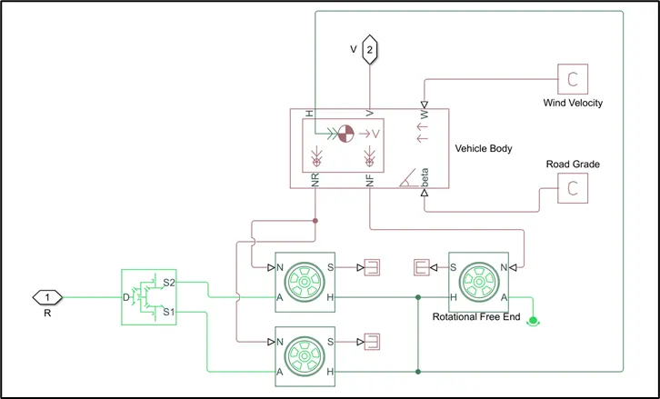

   Fig.14. Vehicle Subsystem

   
   - Differential Block
   The Differential block represents a gear mechanism that allows the driven shafts to spin at different speeds. Differentials are common in automobiles, where they enable the various wheels to spin at different speeds while cornering. Ports D, S1, and S2 represent the longitudinal driveshaft and the sun gear shafts of the differential, respectively. Any one of the shafts can drive the other two.
   
   D — Driveshaft (Rotational mechanical conserving port associated with the longitudinal driveshaft)
   S1 — Sun gear 1 (Rotational conserving port associated with sun gear 1)
   S2 — Sun gear 2 (Rotational conserving port associated with sun gear 2)
   
   As per the model parameters, the value for the gear ratio is set to 1 since the drive is direct.
   
   - Tire (Magic Formula) Blocks
   

   The Tire (Magic Formula) block models a tire with longitudinal behavior given by the Magic Formula [1], an empirical equation based on four fitting coefficients. The block can model tire dynamics under constant or variable pavement conditions.

   The longitudinal direction of the tire is the same as its direction of motion as it rolls on the pavement. This block is a structural component based on the Tire-Road Interaction (Magic Formula) block.

   To increase the fidelity of the tire model, you can specify properties such as tire compliance, inertia, and rolling resistance. However, these properties increase the complexity of the tire model and can slow down the simulation. Consider ignoring tire compliance and inertia if simulating the model in real-time or if preparing the model for hardware-in-the-loop (HIL) simulation.
   For our model, we utilize 4 of these blocks to simulate the wheels of the car. Each block is configured with the same values as mentioned in the parameters section. Also, the front and rear tires are connected in pairs respectively. The gear is connected with the front axle for power delivery.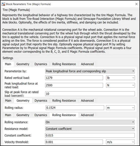

   Fig.15. Tire Block Configuration

   
   - Vehicle Body Block
   

   The Vehicle Body block represents a two-axle vehicle body in longitudinal motion. The vehicle can have the same or a different number of wheels on each axle. For example, two wheels on the front axle and one wheel on the rear axle. The vehicle wheels are assumed identical in size. The vehicle can also have a center of gravity (CG) that is at or below the plane of travel.

   The block accounts for body mass, aerodynamic drag, road incline, and weight distribution between axles due to acceleration and road profile. Optionally include pitch and suspension dynamics. The vehicle does not move vertically relative to the ground.
   In the block, we input all the necessary values as mentioned in the parameters section. The Tire blocks are connected with the respective ports.
   
   W — Headwind speed, m/s (Physical signal input port for headwind speed)
   beta — Road incline angle, rad (Physical signal input port for road incline angle)
   V — Longitudinal velocity, m/s (Physical signal output port for vehicle longitudinal velocity)
   NF — Front axle normal force, N (Physical signal output port for normal force on the front axle. Wheel forces are considered positive if acting downwards)
   NR — Rear-axle normal force, N (Physical signal output port for normal force on the rear axle. Wheel forces are considered positive if acting downwards)
   H — Horizontal motion (Conserving port associated with the horizontal motion of the vehicle body. All tires are connected to this port)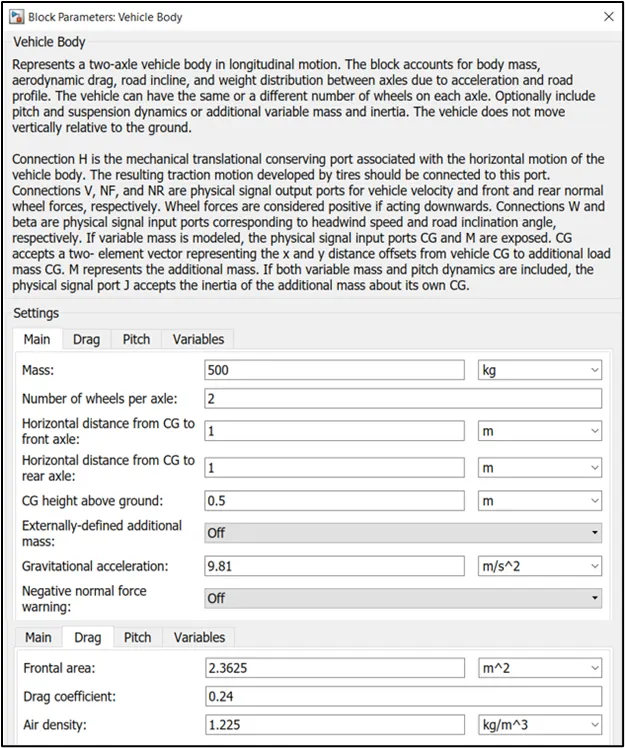

   Fig.16. Vehicle Body Block Configuration

   
   [F] Battery Subsystem:
   

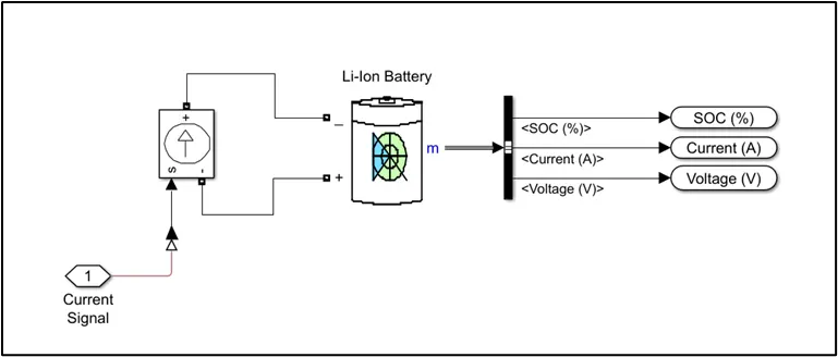
   Fig.17. Battery Subsystem

   
   - Controlled Current Source Block:
   

   The Controlled Current Source block converts the Simulink input signal into an equivalent current source. The generated current is driven by the input signal of the block. The positive current direction is as shown by the arrow in the block icon.

   The positive direction of the current flow is indicated by the arrow.
   The current signal from the control system determines how this current source behaves with how much flow of current.
   
   - Battery Block:
   The Battery block implements a generic dynamic model that represents the most popular types of rechargeable batteries.
   
   

   For the lithium-ion battery type, the model uses these equations.

   • Discharge Model (i* > 0)

   `f_1 (it,i∗,i)=E_0 −K⋅ Q/( Q−it) ⋅i∗−K⋅ Q /(Q−it) ⋅it+A⋅exp(−B⋅it)`
   

   • Charge Model (i* < 0)

   `f_2(it,i∗,i)=E_0−K⋅Q/(it+0.1⋅Q)⋅i∗−K⋅Q/(Q−it)⋅it+A⋅exp(−B⋅it)`
   
   m — Battery temperature, state-of-charge, current, voltage, age, maximum capacity, and ambient temperature (Output vector of signals for the battery temperature, state-of-charge, current, voltage, age, maximum capacity, and the ambient temperature)

   Battery SOC is represented as a percentage (between 0 and 100%). The SOC is 100% for a fully charged battery and 0% for an empty battery. The SOC is calculated as:

   `SOC=100(1−1/Qint_0^ti(t).dt)`

   
   As per the given data for the battery pack of Treo-SFT, the capacity for it is 7.37 kWh operating at 48V. This means that the Ampere-hour rating is 153.54 AHr. These values are added to the block.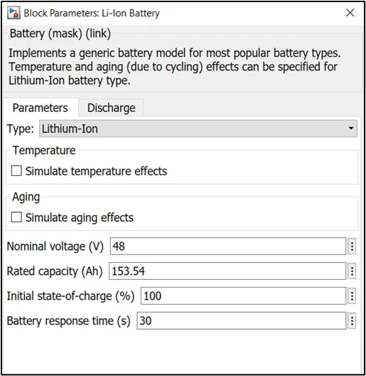

   Fig.18. Battery Block Configuration

   
   

   [G] Energy Consumption Estimation Subsystem:
   

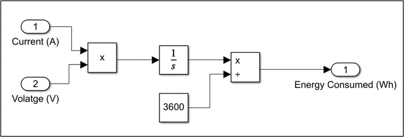
   Fig.19. Energy Consumption Estimation Subsystem

   
   The above subsystem is the Energy estimate block, where the product of Voltage and Current is integrated and divided by 3600 to get the Energy Consumed in Wh. This arrangement gives us the Energy consumed by the battery.
   
3. Results:-
   
   In this project, we have evaluated three results which go as follows for the respective drive cycles:
   
   I. HWFET (765 seconds)
   
   A. Actual Speed vs. Drive Cycle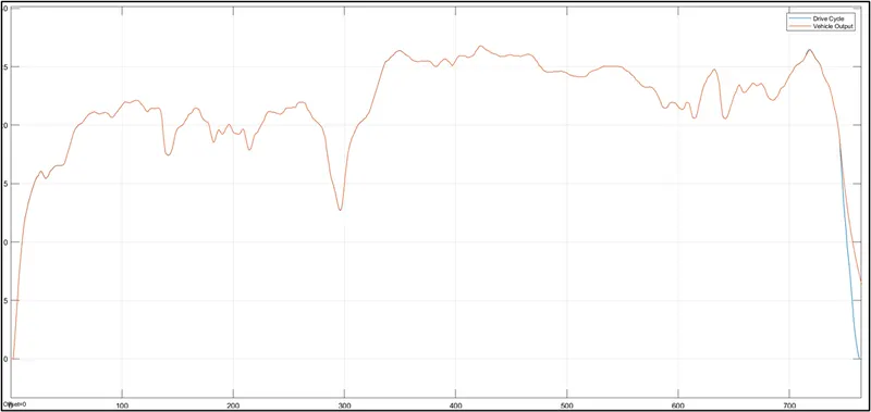

   Fig.20. Plot for Actual Speed vs. Drive Cycle

   
   From the above plot, it is evident that with the given model parameters and configuration, our model can handle the drive cycle conditions in this case. The model can mimic the drive cycle perfectly until the final deceleration stage where the vehicle takes time to slow down. We can observe that model traces the plot efficiently during acceleration and constant speeds. There are slight inconsistencies during the deceleration phases due to the regenerative braking effect.
   
   B. Battery data (SoC and Energy Consumption)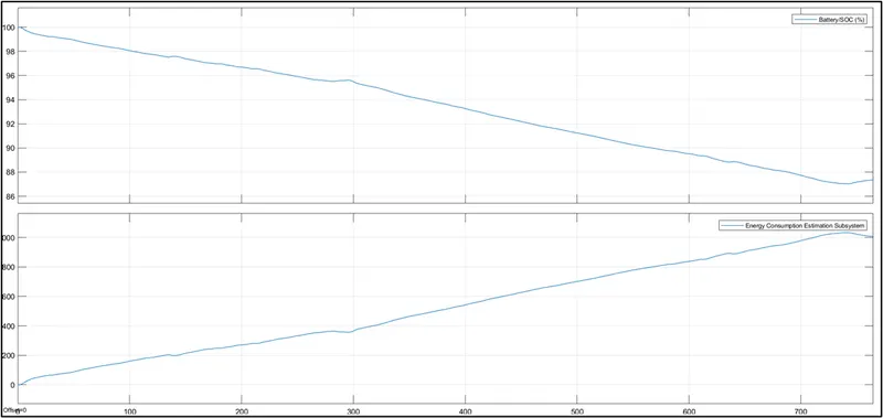

   Fig.21. Plot for the Battery Statistics

   
   From the above plot, we can study the battery behavior for the given conditions. In general, with this drive cycle, the battery is depleted by approximately 13%. We can see that during deceleration phases, the battery is being charged due to regenerative braking. Since we haven't tuned the regenerative braking, the program uses default settings to charge the battery.
   While the vehicle completes the cycle, the system uses about 1 kWh of battery which again reduces at the end due to charging.
   
   C. Thermal behavior of Controller and DC Motor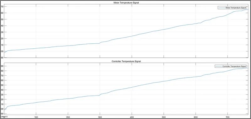

   Fig.22. Plot for the Thermal statistics

   
   The thermal behaviors are captured for the motor and the controller. On the top half, we have the motor temperature data which shows that while operating the motor temperature starts increasing from 25ºC to 92ºC. This happens majorly due to the I²R losses in the stator windings.
   On the bottom half, we have the controller temperature data which shows that during operation the controller temperature starts increasing from 25ºC to 112ºC. The cause of this is high switching losses in the H-bridge.
   These values are depending on the assumed values of Thermal masses we have provided for both of the components.
   It goes to show that the temperature of the EV components has to be kept under control to avoid any further loss in efficiency and worst-case failures.
   
   D. Distance traveled by the Vehicle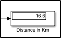

   Fig.23. Total distance traveled

   
   Our vehicle model traversed a distance of 16.6 KM with the HWFET drive cycle.
   
   II. EUDC (400 seconds)
   
   A. Actual Speed vs. Drive Cycle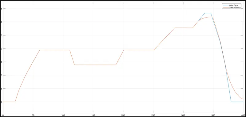

   Fig.24. Plot for Actual Speed vs. Drive Cycle

   
   From the above plot, it is evident that with the given model parameters and configuration, our model can handle the drive cycle conditions in this case. The model fails to trace the drive cycle at higher speeds, presumably due to low motor speed or low power to cope with the speed. Other than that, the model works as speculated.
   
   B. Battery data (SoC and Energy Consumption)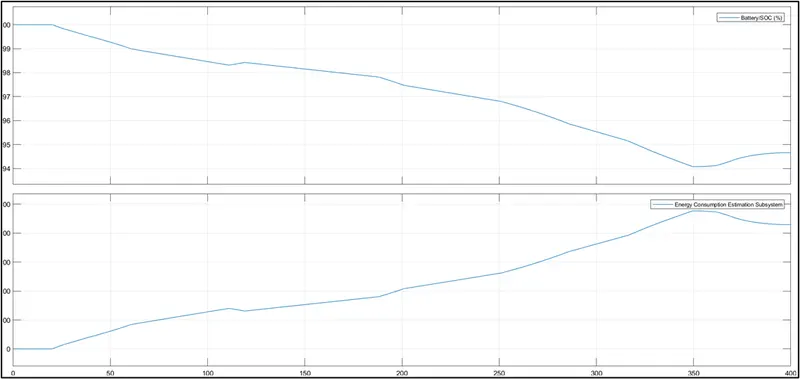

   Fig.25. Plot for the Battery Statistics

   
   From the above plot, we can study the battery behavior for this drive cycle. The battery is depleted by approximately 6%. We can see that during the deceleration phase at the end of the cycle, the battery is being charged due to regenerative braking and increases the final SoC to 94.7%.
   While the vehicle completes the cycle, the system uses about 490 Wh of battery energy which again reduces at the end due to charging.
   
   C. Thermal behavior of Controller and DC Motor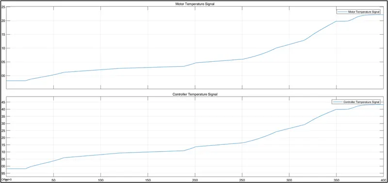

   Fig.26. Plot for the Thermal statistics

   
   The thermal behaviors are captured for the motor and the controller. On the top half, we have the motor temperature data which shows that while operating the motor temperature starts increasing from 25ºC to 49.5ºC.
   On the bottom half, we have the controller temperature data which shows that during operation the controller temperature starts increasing from 25ºC to 70ºC.
   Since the drive cycle is not too long, the temperatures of the components stay within the workable limits.
   
   D. Distance traveled by the Vehicle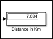

   Fig.27. Total distance traveled

   
   Our vehicle model traversed a distance of 7.034 KM with the EUDC drive cycle.
   
   III. Japanese 10 Mode (135 seconds)
   
   A. Actual Speed vs. Drive Cycle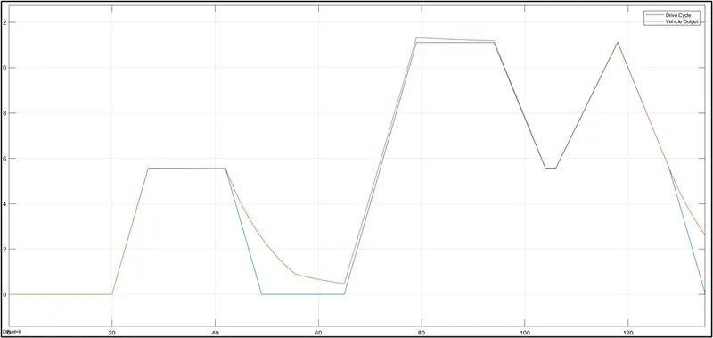

   Fig.28. Plot for Actual Speed vs. Drive Cycle

   
   From the above plot, it is evident that with the given model parameters and configuration, our model can handle the drive cycle conditions in this case but cannot perfectly trace the deceleration path. This can be due to lower resistance from the motor during the regenerative stage. This can allow us to rework the model for this drive cycle. Since this drive cycle is a low-speed one, which might be the most frequent cycle if the E-rickshaw is being operated commercially in busy city traffic.
   
   B. Battery data (SoC and Energy Consumption)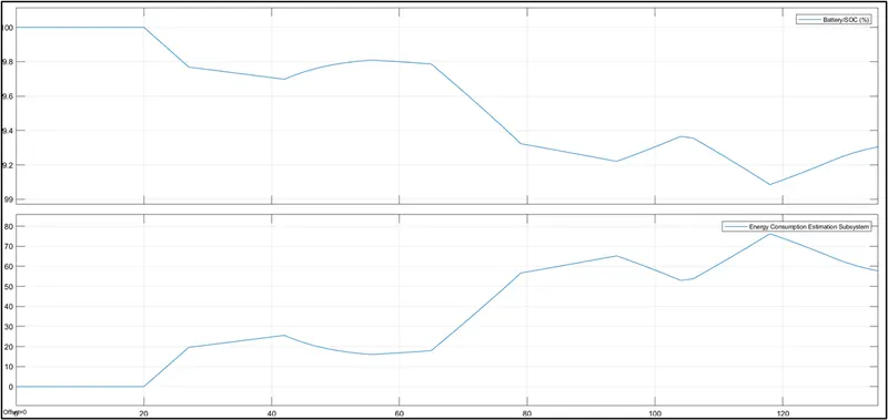

   Fig.29. Plot for the Battery Statistics

   
   From the above plot, we can study the battery behavior for this drive cycle. The battery is depleted by a mere 0.9%. We can see that during the deceleration phases, the battery is being charged due to regenerative braking and increases the final SoC to 99.3%.
   While the vehicle completes the cycle, the system uses a maximum of 76 Wh of battery energy which again reduces to 69 Wh at the end due to charging. This cycle consumes the least amount of battery energy due to low distance and speed.
   
   C. Thermal behavior of Controller and DC Motor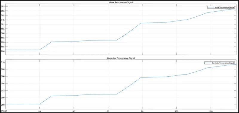

   Fig.30. Plot for the Thermal statistics

   
   The thermal behaviors are captured for the motor and the controller. On the top half, we have the motor temperature data which shows that while operating the motor temperature starts increasing from 25ºC to 29.5ºC.
   On the bottom half, we have the controller temperature data which shows that during operation the controller temperature starts increasing from 25ºC to 36.35ºC.
   Since the drive cycle is short, the temperatures of the components do not heat up as much.
   
   D. Distance traveled by the Vehicle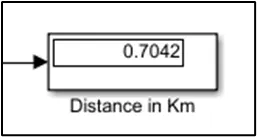

   Fig.31. Total distance traveled

   
   Our vehicle model traversed a distance of 0.7042 KM with the Japanese Mode 10 drive cycle.
   
   
4. Conclusion:-
   
   The following points are drawn as conclusions from this project:
   

   An Electric Rickshaw (3-Wheeler) powertrain model was designed and the required parameters and results were documented. From the simulation results, it is clear that if we can't exactly get the real-time results, we can still serve the purpose by considering the assumptions. There lies a lot of scope for improvement in the model. For example, due to the high temperatures of the components in the first drive cycle, the model could utilize a thermal management system to keep the components under working limits. Satisfactory results were acquired from the model in terms of the parameters assumed.

   
   

IV. REFERENCES

1. Shakti Foundation - Handbook: E-Rickshaw Deployment in Indian Cities
2. Mahindra Electric Website - Mahindra Treo E Rickshaw Webpage
3. MathWorks Help - Simulink Documentation - MathWorks India
4. Chalmer's University Student Thesis - EmmaGrunditz_PhDthesis_lowrez.pdf (chalmers.se)