Final Project: Electric Rickshaw modelling
AIM:- To model Electric Rickshaw(three-wheel passenger vehicle) with help of MATLAB and SIMULINK.
OBJECTIVES:-
1) Creating a detailed MATLAB model of an electric rickshaw.
2) Making an excel sheet of all input and assumed data.
3)creating a detailed report of electric rickshaw modeling.
***************************************************************************************
HISTORY:-
Auto rickshaw
An auto-rickshaw is a motorized version of the pulled rickshaw or cycle rickshaw. Most have three wheels and do not tilt. They are known by many terms in various countries including auto, auto/auto-rickshaw, baby taxi, pigeon, bajaj, chand gari, Lapa, tuk-tuk, Keke-napep, 3wheel, Pragya, bao-bao, or tukxi.
An auto-rickshaw is a common form of urban transport, both as a vehicle for hire and private use, in many countries around the world. They are especially common in countries with tropical or subtropical climates, since they usually are not fully enclosed, and in many developing countries because they are relatively inexpensive to own and operate. As of 2019, Bajaj Auto of Pune, India is the world's largest auto rickshaw manufacturer, selling 780,000 during the fiscal year.[1]
There are many different auto rickshaw designs. The most common type is characterized by a sheet-metal body or open-frame resting on three wheels; a canvas roof with drop-down side curtains; a small cabin at the front for the driver (in India, the auto-wallah or Tuk Tuk-wallah), with handlebar controls; and a cargo, passenger, or dual-purpose space at the rear. Another common type is a motorcycle that has an expanded sidecar or, less often, is pushing or pulling a passenger compartment.
Origin
In the 1930s Japan, which was the most industrialized country in East Asia at the time, encouraged the development of motorized vehicles including less expensive three-wheeled vehicles based on motorcycles. The Mazda-Go, a 3-wheel open "truck" released in 1931 is often considered the first of what became auto rickshaws. Later that decade the Japanese Ministry of Posts and Telecommunications of Japan distributed about 20,000 used three-wheelers to Southeast Asia as part of efforts to expand its influence in the region. They became popular in some areas, especially Thailand, which developed local manufacturing and design after the Japanese government abolished the three-wheeler license in Japan in 1965.
Production in Southeast Asia started from the knockdown production of the Daihatsu Midget, which was introduced in 1959.]An exception is the indigenously-modified Philippine tricycle, which originates from the Rikuo Type 97 motorcycle with a sidecar, introduced to the islands in 1941 by the Imperial Japanese Army during World War II.
In Europe, Corradino D'Ascanio, aircraft designer at Piaggio and inventor of the Vespa, came up with the idea of building a light three-wheeled commercial vehicle to power Italy's post-war economic reconstruction. The Piaggio Ape followed suit in 1947.
India
Most cities offer auto rickshaw service, although cycle rickshaws are also common and even hand-pulled rickshaws exist in certain areas such as Kolkata. Many state governments have launched an initiative of a women-friendly rickshaw service called the Pink Rickshaws.
Auto rickshaws are used in cities and towns for short distances; they are less suited to long distances because they are slow and the carriages are open to air pollution.[25]:57,58,110 Auto rickshaws (often called "autos") provide cheap and efficient transportation. Modern auto rickshaws run on compressed natural gas (CNG) and liquified petroleum gas (LPG) due to government regulations and are environmentally friendly compared to full-sized cars.
To augment the speedy movement of traffic, auto rickshaws are not allowed in the southern part of Mumbai.
India is the location of the annual Rickshaw Run.
There are two types of auto-rickshaws in India. In older versions, the engines were below the driver's seat, while in newer versions engines are in the rear. They normally run on petrol, CNG, or diesel. The seating capacity of a normal rickshaw is four, including the driver's seat. Six-seater rickshaws exist in different parts of the country, but the model was officially banned in the city of Pune on 10 January 2003 by the Regional Transport Authority (RTA).
CNG autos in many cities (e.g. Delhi, Agra) are distinguishable from the earlier petrol-powered autos by a green and yellow livery, as opposed to the earlier black and yellow appearance. In other cities (such as Mumbai) the only distinguishing feature is the 'CNG' print found on the back or side of the auto. Some local governments are considering four-stroke engines instead of two-stroke versions.[citation needed]
Auto rickshaw manufacturers in India include Bajaj Auto, Atul Auto Limited, Oculus Auto,[29] Kerala Automobiles Limited, Force Motors, Mahindra & Mahindra, Piaggio Ape, TVS Motors, and Fleek Motors.
In Delhi, there also used to be a variant powered by a Harley-Davidson engine called the phat-phati, because of the sound it made. The story goes that shortly after Independence a stock of Harley-Davidson motorbikes was found that had been used by British troops during World War II and left behind in a military storage house in Delhi. Some enterprising drivers purchased these bikes, added on a gearbox (probably from a Willys jeep), welded on a passenger compartment that was good for four to six passengers, and put the unconventional vehicles onto the roads. A 1998 ruling of the Supreme Court against the use of polluting vehicles finally signed the death warrant of Delhi's phat-phatis.
- As of 2018, India has about 1.5 million battery-powered, three-wheeled rickshaws on its roads. Some 11,000 new ones hit the streets each month, creating a US$1.5 billion market. Manufacturers include Mahindra & Mahindra Ltd. and Kinetic Engineering. A hindrance to the adoption of electric vehicles is the paucity of charging stations; India had only 425 at year-end 2017. By 2022 the number is projected to rise to 2,800.
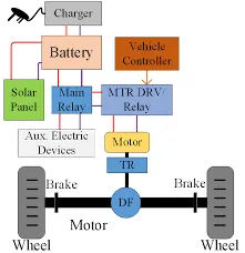
Important factors and construction of E-Rickshaw
The electric rickshaw has been global since the 1940s from the time of post era. But, its utilization and popularity have actually come into prominence in the last 4-5 years. Actually, the concept of tricycles with fuel run emerged at that time, after that the auto-rickshaws have dominated the market. It is only in the year 2008 that battery-operated rickshaws gain much importance worldwide.
Construction of E-Rickshaw
No doubt that a battery-operated vehicle is robust and strong enough. Also, it is ensured that this vehicle provides all the facilities for the comfort of every passenger. No doubt there is a hell of a lot of E-Rickshaw spare parts required for the construction of e-rickshaw. Also, the vehicle is crafted with the best quality of metal and fiberglass. Among the other materials, an open frame is used for the construction of these e-rickshaws. The rickshaw is no doubt cost-effective because it is battery-operated as well as consumes less energy.
The 3 wheeler E- rickshaw is definitely the best substitute for fuel-driven vehicles and efficient when comes to battery power. Also, there is no emission of harmful pollutants from this vehicle so it helps to increase the durability and strengthens the vehicle. The materials which are used in constructing the vehicle such as fiberglass help it to make the vehicle more efficient. Also, this vehicle is absolutely perfect to cover the short distance as well as carry small loads.
How does the Vehicle Work?
The bodyweight of the E- rickshaw is extremely light and because of that durability of the battery does not get decreased. The main elements that actually drive the electric rickshaw are a motor, controller, harness, and most importantly its throttle. To get the best service and to increase the benefits from this vehicle these elements are essential.
The motor of the battery generally varies from 650w to 1250 while according to the rules the unit should not increase 650 W. Moreover, these E-rickshaws constitute leaf spring suspension. The power supplies at the rate of 48 V which can also be controlled by a specific controller. Manufacturers must use the superior quality battery to get the best performance and takes care that the batteries don’t get overheated very fast.
The best part of this rickshaw is that they need minimal maintenance. Although it is important that at regular intervals the vehicle must be taken to the service centers. Any misuse of the vehicle might affect the entire system. Also, wrong adjustments with the brakes might affect the motor and other essential elements. If this happens then not only it will severely affect the vehicle but also decrease the mileage.
***************************************************************************************
SIMULINK MODEL:-
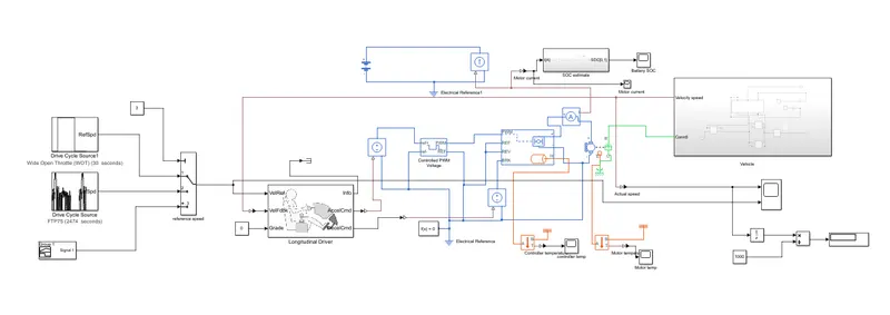
the solver used: auto(ode23t)
Drive cycle source and switch:-
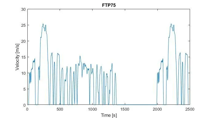
1)FTP75
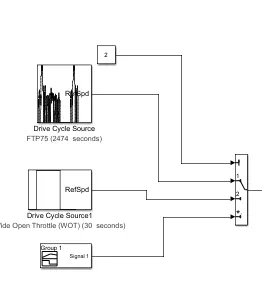
Here we used three drive cycle sources with a multiport switch to select cycle as per our need,
Standard or specified longitudinal drive cycle
- Library:
Powertrain Blockset / Vehicle Scenario Builder
Vehicle Dynamics Blockset / Vehicle Scenarios / Drive Cycle and Maneuvers
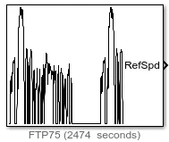
Description
The Drive Cycle Source block generates a standard or user-specified longitudinal drive cycle. The block output is the specified vehicle longitudinal speed, ts2
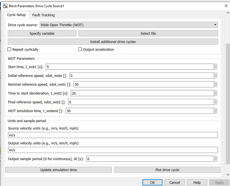
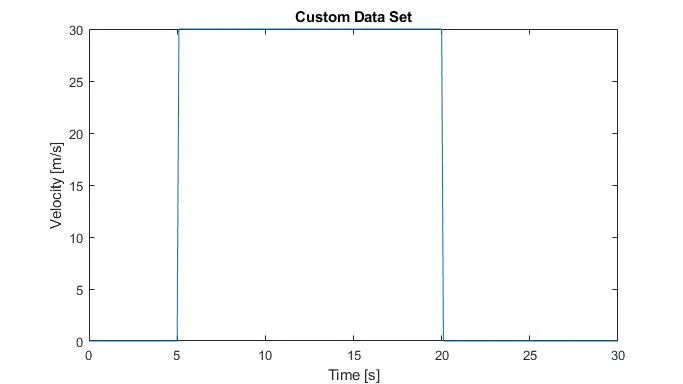
2)Wide open throttle:-
kept parameters by default
Custome cycle source:-
we used signal builder for that,
3)Signal Builder
Create and generate interchangeable groups of signals whose waveforms are piecewise linear
- Library: Simulink / Sources
Description
The Signal Builder block allows you to create interchangeable groups of piecewise linear signal sources and use them in a model. You can quickly switch the signal groups into and out of a model to facilitate testing. In the Signal Builder window, create signals and define the output waveforms.
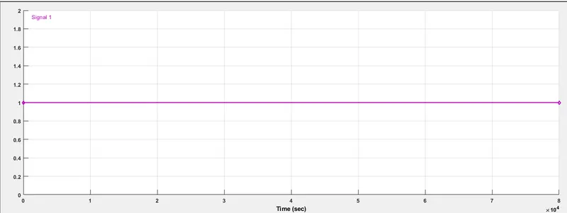
and set the y axis to 12.5 because we wanted to our vehicle with a constant speed of 45 kmph which is 12.5 in m/s for 100 km which takes time about 80000 seconds as our x-axis
but we took a scale where we kept 12.5 as 1 so in the final distance calculation we will multiply our distance output with 12.5
To implement these three drive cycle together we are using
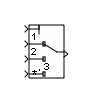
Multiport Switch
- Library:
Simulink / Signal Routing
HDL Coder / Signal Routing
Description
The Multiport Switch block determines which of several inputs to the block passes to the output. The block bases this decision on the value of the first input. The first input is the control input and the remaining inputs are the data inputs. The value of the control input determines which data input passes to the output.
***********************************************************************************
Longitudinal speed-tracking controller
- Library:
Powertrain Blockset / Vehicle Scenario Builder
Vehicle Dynamics Blockset / Vehicle Scenarios / Driver
Description
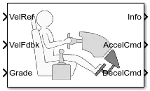
The Longitudinal Driver block implements a longitudinal speed-tracking controller. Based on reference and feedback velocities, the block generates normalized acceleration and braking commands that can vary from 0 through 1. You can use the block to model the dynamic response of a driver or to generate the commands necessary to track a longitudinal drive cycle.
-the changes we made,
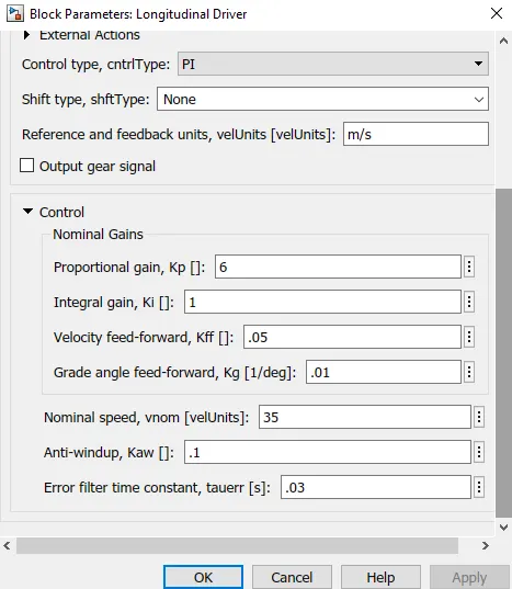
, and keeping all other values by default
-External actions:-PI
-Shift type:-None
-Reference and feedbacks units, VelUnits:-m/s
***************************************************************************************************
Power controller and motor block:-
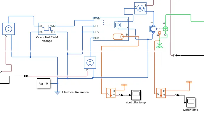
i )Controlled PWM Voltage
Pulse-width modulated voltage source
Library:
Simscape / Electrical / Integrated Circuits
Description
The Controlled PWM Voltage block represents a pulse-width modulated (PWM) voltage source. The block has two modeling variants, accessible by right-clicking the block in your block diagram and then selecting the appropriate option from the context menu, under Simscape > Block choices:
Electrical input ports — The block calculates the duty cycle based on the reference voltage across its ref+ and ref- ports. This modeling variant is the default.
PS input — Specify the duty cycle value directly by using an input physical signal port.
For the Electrical input ports variant of the block, the demanded duty cycle is
100∗Vref−VminVmax−Vmin percent
where:
Vref is the reference voltage across the ref+ and ref- ports.
Vmin is the minimum reference voltage.
Vmax is the reference voltage.
-the changes we made,
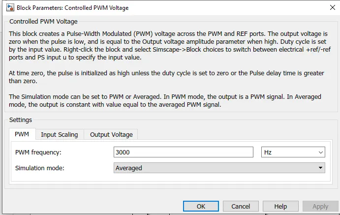
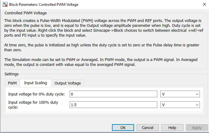
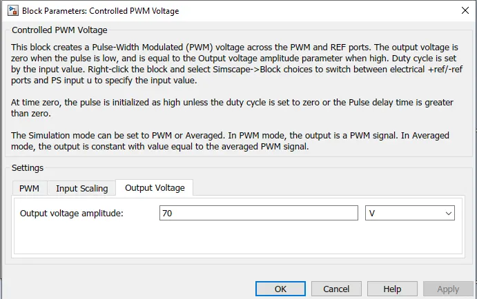
, and keeping all other values by default
ii) H-Bridge
H-bridge motor driver
Library:
Simscape / Electrical / Semiconductors & Converters / Converters
Description
The H-Bridge block represents an H-bridge motor driver. The block has the following two Simulation mode options:
PWM — The H-Bridge block output is a controlled voltage that depends on the input signal at the PWM port. If the input signal has a value greater than the Enable threshold voltage parameter value, the H-Bridge block output is on and has a value equal to the value of the Output voltage amplitude parameter. If it has a value less than the Enable threshold voltage parameter value, the block maintains the load circuit using one of the following three Freewheeling mode options:
Via one semiconductor switch and one freewheeling
                                diode
Via two freewheeling diodes
Via two semiconductor switches and one freewheeling
                                diode
The first and third options are sometimes referred to as asynchronous operations.
The signal at the REV port determines the polarity of the output. If the value of the signal at the REV port is less than the value of the Reverse threshold voltage parameter, the output has positive polarity; otherwise, it has negative polarity.
VO is the value of the Output voltage amplitude parameter.
VPWM is the value of the voltage at the PWM port.
APWM is the value of the PWM signal amplitude parameter.
IOUT is the value of the output current.
RON is the Bridge on the resistance parameter.
Averaged — This mode has two Load current characteristics options:
Smoothed
Unsmoothed or discontinuous
The Smoothed the option assumes that the current is practically continuous due to load inductance. In this case, the H-Bridge block output is:
VOVPWMAPWM−IOUTRON
where:
iii)Thermal Port
The block has an optional thermal port, hidden by default. To expose the thermal port, right-click the block in your model, and then from the context menu select Simscape > Block choices > Show thermal port. This action displays the thermal port H on the block icon and adds the Temperature Dependence and Thermal Port parameters. These parameters are described further on this reference page.
When the thermal port is visible:
The heat generated by the bridge on-resistance and freewheeling diodes is added to the thermal port. The thermal port has an associated thermal mass and initial temperature that you can set from the Thermal Port parameters.
The bridge on-resistance and freewheeling diode resistance become functions of temperature. You can define the values for these resistances and the second measurement temperature from the Temperature Dependence parameters. Resistance is assumed to vary linearly between the two measurement temperatures. Extrapolation is used for temperatures outside of this range, except for when simulating in averaged mode with discontinuous load current characteristics.
-the changes we made,
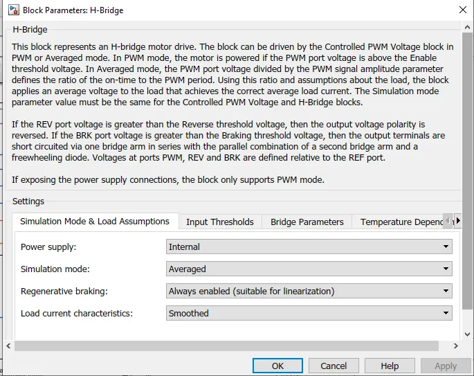
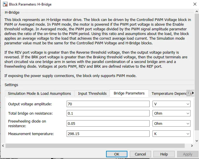
, and keeping all other values by default
we kept all parameters by default
iv)DC Motor
DC motor model with electrical and torque characteristics and fault modeling
- Library:
Simscape / Electrical / Electromechanical / Brushed Motors
Description
The DC Motor block represents the electrical and torque characteristics of a DC motor using the following equivalent circuit model:
You specify the equivalent circuit parameters for this model when you set the Model parameterization parameter to By equivalent
circuit parameters. The resistor R corresponds to the resistance you specify in the Armature resistance parameter. The inductor L corresponds to the inductance you specify in the Armature inductance parameter.
the procedure which we follow to add a thermal port to H-bridge here we will be going to do the same for DC motor
the changes we made,
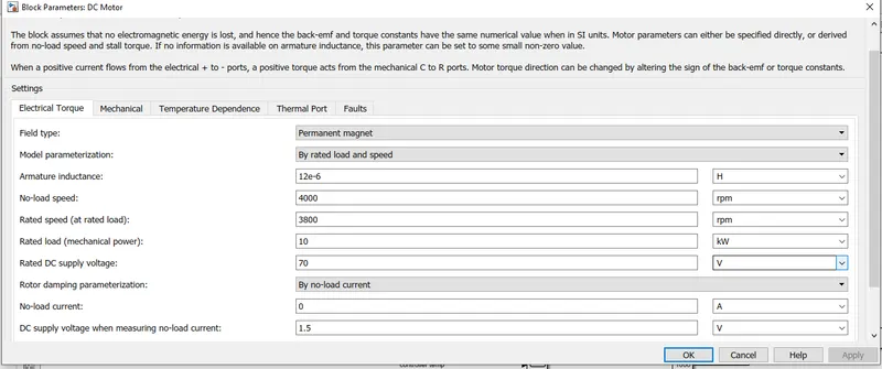
v)Controlled Voltage Source
The ideal voltage source is driven by input signal
Library
Electrical Sources
Description
The Controlled Voltage Source block represents an ideal voltage source that is powerful enough to maintain the specified voltage at its output regardless of the current flowing through the source. The output voltage is V = Vs, where Vs is the numerical value presented at the physical signal port.
v)Temperature Sensor
Ideal temperature sensor
Library
vi)Thermal Sensors
Description
The Temperature Sensor block represents an ideal temperature sensor, that is, a device that determines the temperature differential measured between two points without drawing any heat.
Connections A and B are thermal conserving ports that connect to the two points where the temperature is being monitored. Port T is a physical signal port that outputs the temperature differential value.
The block positive direction is from port A to port B. The measured temperature is determined as T = TA – TB.
vii)Current Sensor
The current sensor in electrical systems
Library
Electrical Sensors
Description
The Current Sensor block represents an ideal current sensor, that is, a device that converts current measured in any electrical branch into a physical signal proportional to the current.
Connections + and – are electrical conserving ports through which the sensor is inserted into the circuit. The connection I am a physical signal port that outputs the measurement result.
viii)Electrical Reference
Connection to electrical ground
Library
Electrical Elements
Description
The Electrical Reference block represents an electrical ground. Electrical conserving ports of all the blocks that are directly connected to the ground must be connected to an Electrical Reference block. A model with electrical elements must contain at least one Electrical Reference block.
ix)Solver Configuration
Physical Networks environment and solver configuration
Library
Utilities
Description
Each physical network represented by a connected Simscape™ block diagram requires solver settings information for simulation. The Solver Configuration block specifies the solver parameters that your model needs before you can begin the simulation.
Each topologically distinct Simscape block diagram requires exactly one Solver Configuration block to be connected to it.
x) Thermal Reference
Reference connection for thermal ports
Library
Thermal Elements
Description
The Thermal Reference block represents a thermal reference point, that is, a point with an absolute zero temperature, concerning which all the temperatures in the system are determined.
***************************************************************************************
Battery package:-
Behavioral battery model
- Library:
- Simscape / Electrical / Sources
Description
The Battery block represents a simple battery model. The block has four modeling variants, accessible by right-clicking the block in your block diagram and then selecting the appropriate option from the context menu, under Simscape > Block choices:
Uninstrumented | No thermal port — A basic model that does not output battery charge level or simulates thermal effects. This modeling variant is the default.
Uninstrumented | Show thermal port — Model with exposed thermal port. This model does not measure the internal charge level of the battery.
Instrumented | No thermal port — Model with an exposed charge output port. This model does not simulate thermal effects.
Instrumented | Show thermal port — Model that lets you measure the internal charge level of the battery and simulate thermal effects. Both the thermal port and the charge output port are exposed.
-the changes we made,
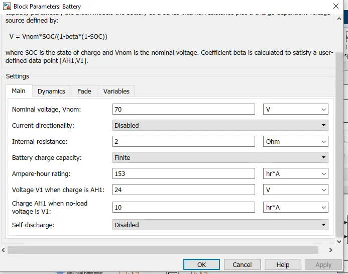
-by keeping all other values as default,
The ideal current source is driven by input signal
ii)Controlled Current Source
Library
Electrical Sources
Description
The Controlled Current Source block represents an ideal current source that is powerful enough to maintain the specified current through it regardless of the voltage across the source.
The output current is I = Is, where Is is the numerical value presented at the physical signal port.
The positive direction of the current flow is indicated by the arrow.
SOC ESTIMATE:-
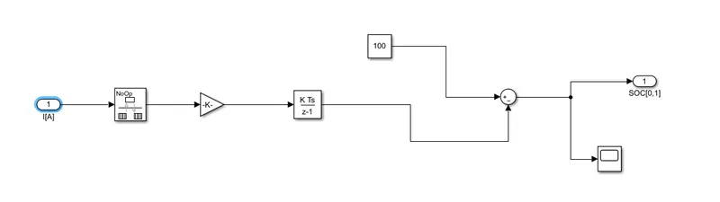 i)Rate Transition
- Library:
Simulink / Signal Attributes
HDL Coder / Signal Attributes

Description
The Rate Transition block transfers data from the output of a block operating at one rate to the input of a block operating at a different rate. Use the block parameters to trade data integrity and deterministic transfer for faster response or lower memory requirements. To learn about data integrity and deterministic data transfer, see Data Transfer Problems (Simulink Coder).
ii)Gain
Multiply input by constant
- Library:
Simulink / Commonly Used Blocks
Simulink / Math Operations
HDL Coder / Commonly Used Blocks
HDL Coder / HDL Floating Point Operations
HDL Coder / Math Operations

Description
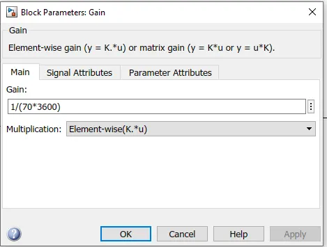
The Gain block multiplies the input by a constant value (gain). The input and the gain can each be a scalar, vector, or matrix.
You specify the value of gain in the Gain parameter. The Multiplication parameter lets you specify element-wise or matrix multiplication. For matrix multiplication, this parameter also lets you indicate the order of the multiplicands.
Gain is converted from doubles to the data type specified in the block mask offline using round-to-nearest and saturation. The input and gain are then multiplied, and the result is converted to the output data type using the specified rounding and overflow modes.
iii)Discrete-Time Integrator
- Library:
Simulink / Commonly Used Blocks
Simulink / Discrete
HDL Coder / Discrete
HDL Coder / HDL Floating Point Operations

Description
Use the Discrete-Time Integrator block in place of the Integrator block to create a purely discrete model. With the Discrete-Time Integrator block, you can:
Define initial conditions on the block dialog box or as input to the block
Define an input gain (K) value
Output the block state
Define upper and lower limits on the integral
Reset the state with an additional reset input
************************************************************************************
Vehicle body and Transmission
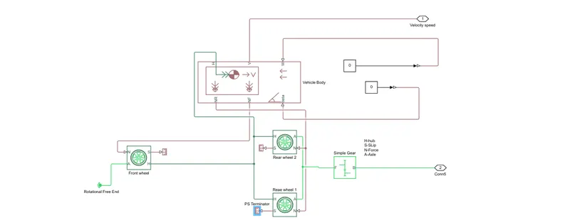 i)Vehicle Body
A two-axle vehicle with longitudinal dynamics and motion and adjustable mass, geometry, and drag properties
- Library:
Simscape / Driveline / Tires & Vehicles
Description
The Vehicle Body block represents a two-axle vehicle body in longitudinal motion. The vehicle can have the same or a different number of wheels on each axle. For example, two wheels on the front axle and one wheel on the rear axle. The vehicle wheels are assumed identical in size. The vehicle can also have a center of gravity (CG) that is at or below the plane of travel.
The block accounts for body mass, aerodynamic drag, road incline, and weight distribution between axles due to acceleration and road profile. Optionally include pitch and suspension dynamics. The vehicle does not move vertically relative to the ground.
The block has an option to include an externally-defined mass and externally-defined inertia. The mass, inertia, and center of gravity of the vehicle body can vary over the course of simulation in response to system changes.\
the changes we made,
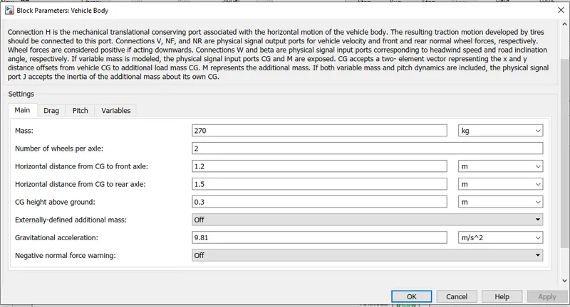
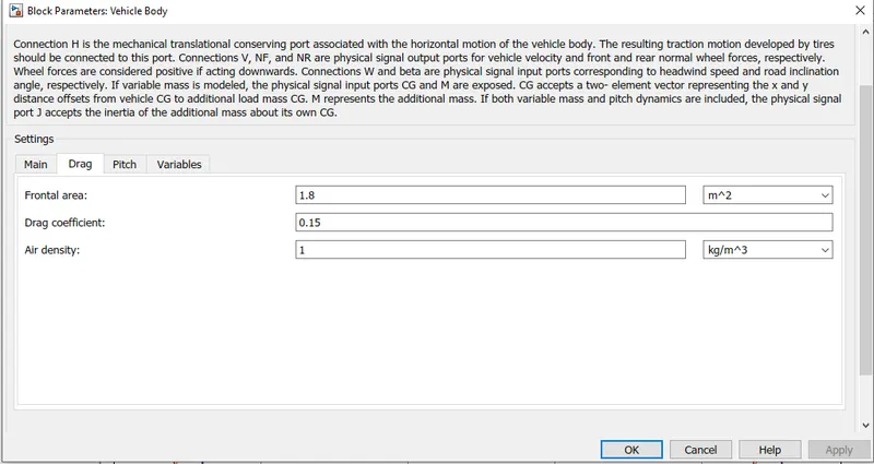
-by keeping all other values as default.
Assumed parameters:-
settings
ii)Tire (Magic Formula)
A tire with longitudinal behavior given by Magic Formula coefficients
- Library:
Simscape / Driveline / Tires & Vehicles
Description
The Tire (Magic Formula) block models a tire with longitudinal behavior given by the Magic Formula [1], an empirical equation based on four fitting coefficients. The block can model tire dynamics under constant or variable pavement conditions.
The longitudinal direction of the tire is the same as its direction of motion as it rolls on the pavement. This block is a structural component based on the Tire-Road Interaction (Magic Formula) block.
To increase the fidelity of the tire model, you can specify properties such as tire compliance, inertia, and rolling resistance. However, these properties increase the complexity of the tire model and can slow down the simulation. Consider ignoring tire compliance and inertia if simulating the model in real-time or if preparing the model for hardware-in-the-loop (HIL) simulation.
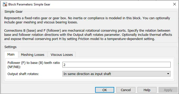
iii)Simple Gear
Simple gear of base and follower wheels with adjustable gear ratio, friction losses, and triggered faults
- Library:
Simscape / Driveline / Gears
Description
The Simple Gear block represents a gearbox that constrains the connected driveline axes of the base gear, B, and the follower gear, F, to corotate with a fixed ratio that you specify. You choose whether the follower axis rotates in the same or opposite direction as the base axis. If they rotate in the same direction, the angular velocity of the follower, ωF, and the angular velocity of the base, ωB, have the same sign. If they rotate in opposite directions, ωF and ωB have opposite signs.
-the changes we made,
*************************************************************************************
Display signals generated during simulation
- Library:
Simulink / Commonly Used Blocks
Simulink / Sinks
HDL Coder / Commonly Used Blocks
HDL Coder / Sinks

Description
The Simulink® Scope block and DSP System Toolbox™ Time Scope block display time-domain signals.
ii)Display
Show value of the input
- Library:
Simulink / Sinks
HDL Coder / Sinks
Description
The Display block shows the value of the input data. You can specify the frequency of the display. For numeric input data, you can also specify the format of the display.
If the block input is an array, you can resize the block vertically or horizontally to show more than just the first element. If the block input is a vector, the block sequentially adds display fields from left to right and top to bottom. The block displays as many values as possible. A black triangle indicates that the block is not displaying all input array elements.
iii)Constant
Generate constant value
- Library:
Simulink / Commonly Used Blocks
Simulink / Sources
DSP System Toolbox / Sources
HDL Coder / Commonly Used Blocks
HDL Coder / Sources

Description
The Constant block generates a real or complex constant value signal. Use this block to provide a constant signal input. The block generates scalar, vector, or matrix output, depending on:
The dimensionality of the Constant value parameter
The setting of the Interpret vector parameters as 1-D parameter
iv)Add, Subtract, Sum of Elements, Sum
Add or subtract inputs
- Library:
Simulink / Math Operations
HDL Coder / HDL Floating Point Operations
HDL Coder / Math Operations

Description
The Sum block performs addition or subtraction on its inputs. The Add, Subtract, Sum of Elements, and Sum blocks are identical blocks. This block can add or subtract scalar, vector, or matrix inputs. It can also collapse the elements of a signal and perform a summation.
v)Divide
- Library:
Simulink / Math Operations
HDL Coder / HDL Floating Point Operations
HDL Coder / Math Operations

Description
The Divide block outputs the result of dividing its first input by its second. The inputs can be scalars, a scalar, and a nonscalar, or two nonscalars that have the same dimensions. This block supports only complex input values at division ports when all ports have the same single or double data type.
vi)Integrator
- Library:
Simulink / Commonly Used Blocks
Simulink / Continuous

Description
The Integrator block outputs the value of the integral of its input signal concerning time.
vii)Simulink-PS Converter
Convert Simulink input signal into a physical signal
Library
Utilities
Description
The Simulink-PS Converter block converts the input Simulink® signal into a physical signal. Use this block to connect Simulink sources or other Simulink blocks to the inputs of a Physical Network diagram.
viii)PS-Simulink Converter
Convert physical signal into Simulink output signal
Library
Utilities
Description
The PS-Simulink Converter block converts a physical signal into a Simulink® output signal. Use this block to connect outputs of a Physical Network diagram to Simulink scopes or other Simulink blocks.
************************************************************************************
RESULTS:-
for Wide-open throttle:-
a)vehicle speed:-
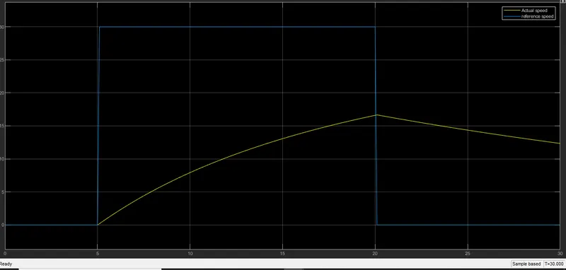
-this graph shows the difference between the ref speed and actual speed when we run the wot drive cycle for 30 second
b) SOC %
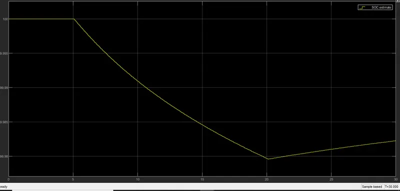
-soc was 100 percent till 5 seconds as the vehicle start accelerating the soc start dropping till the time of 20 sec and when the vehicle goes for deacceleration and soc start get rising.
c) Motor current
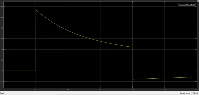
-motor current graph is quite the same as the drive cycle where current demand while the high acceleration point is high and it got decrease when vehicle maintains speed and suddenly it got falls when vehicle completely de-accelerate.
d)controller temperature
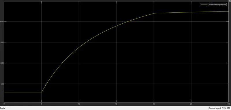
-controller temp is constant till the acceleration starting point and after that, it goes on increasing because the controller working continuously.
e)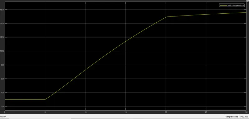
-same with motor temp it stable at initial phase the goes on increasing and the stable at some point
B)1)FTP75
a)Vehicle speed:-
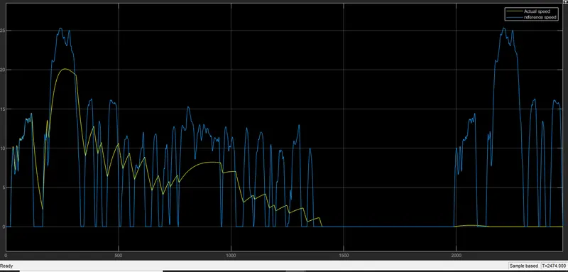
-when we run the model for 2474 sec as its standard time the difference between actual speed and ref speed is higher to match both the speed need change the values of rated load and speed or lowering the vehicle weight
b)SOC%
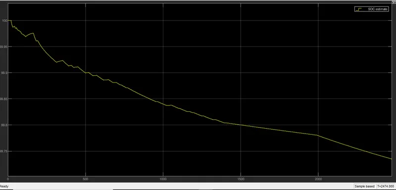
-SOC falling gradually there are some lows and highs which are pretty minor because of the change in vehicle speed continuously.
c)Motor current:-
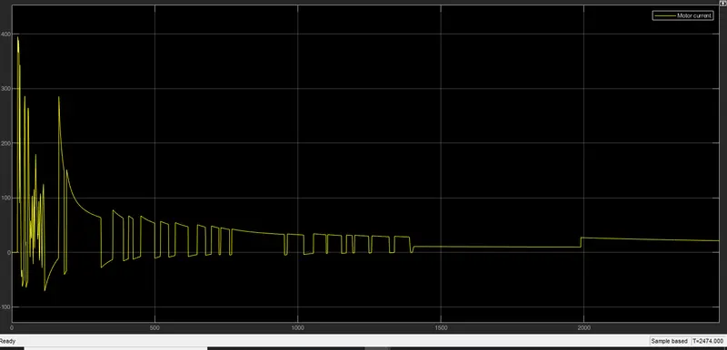
- current fluctuating continuously because of the demanded speed and after a certain point, it became stable.
d) Controller temperature:-
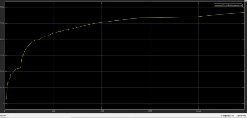
-controller temp keep on rising as its demands are high in the start it increases quickly and then a gradual increment and at the end, the increment is quite smooth
e)Motor temp:-
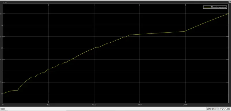
-the motor temp increasing continuously as the motor is working throughout the cycle.
C) Custome data cycle
a)Vehicle speed:-
-here we customize our cycle with the signal builder where we run our vehicle with a constant speed of 45kmph to reach 100 km which calculative needs 8000 seconds.
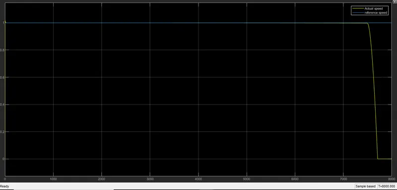
-we can see the difference that reference speed is a constant line but in actual speed increase from zero and after some time and at the end, it started falling till 8000th second.
b)SOC %
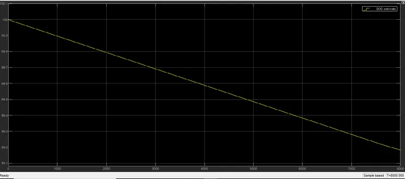
-SOC falling gradually straight line as vehicle speed is constant.
c)Motor current:-
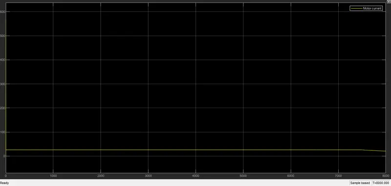
-Motor current is higher at initial because there is the sudden speed in increment but when the vehicle maintains its constant speed and is kept till the end the temperature graph is a straight line.
d)Controller temperature:-
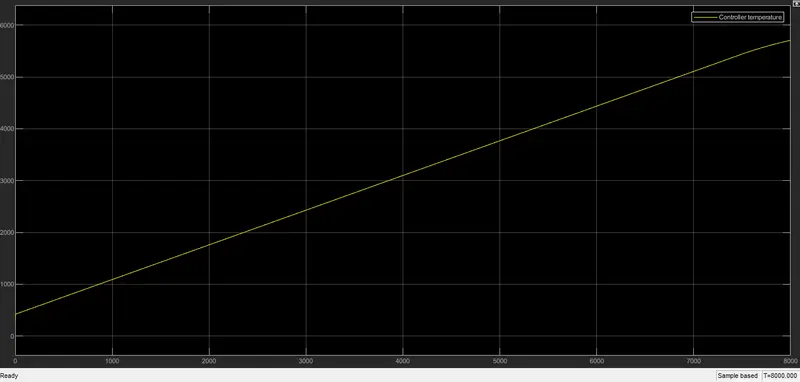
-controller temperature is increasing gradually and the graph line is a smooth inclined line due to constant speed.
e)Motor temperature
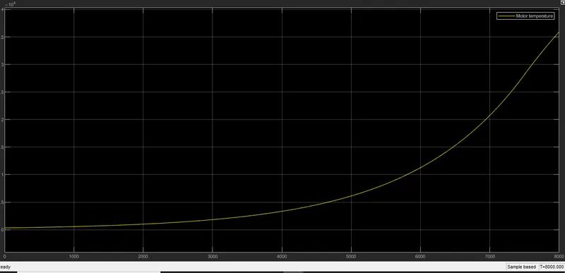
-motor temp graph has a curve line because at the initial stage it is stable and then it increases gradually within less time
f)Distance traveled:-

as we take scale 12.5 as 1 so we will multiply over distance with 12.5 to get the actual distance traveled by vehicle with a constant speed of 45kmph=12.5m/s for 8000 seconds is which is 95.35 km nearby to 100 km
CONCLUSIONS:-
1)In our model we compromised with our motor and controller temperature because since we haven't used any cooling system so values are so high in the real-time vehicle without the cooling system we can't deal with the values of temperature motor and controller as this high
2)hence we completed our model within the given requirement.
3)Also we made some assumptions to perform our simulation and made a data sheet.
4) we also determined all the factor in graphical mannered which describes vehicle performance and we can conclude that electric vehicle is future of automobile industry
REFERENCES:-
1) All the related block and systems studies from:-https://www.mathworks.com/?s_tid=gn_logo
2)Fig1.1DaihatsuMidgetModelDKA:-https://upload.wikimedia.org/wikipedia/commons/thumb/4/4e/1957_Daihatsu_Midget_01.jpg/280px-1957_Daihatsu_Midget_01.jpg
3)Fig 1.2. Schematic diagram of E-rickshaw:-https://encrypted-tbn0.gstatic.com/images?q=tbn:ANd9GcQ2GYUSZvmniayRRT40ZvKD9ifNCL1Gr0Y4r6YEAz5CJ-9J2dmIscBisg7D5yWud-G84ug&usqp=CAU
(Note:- All the related files are attached below)