Final Project: Electric Rickshaw modelling
Aim :
To study a detailed MATLAB model of an electric rickshaw (3 wheel passenger vehicle).
Objective :
Create a detailed MATLAB model of an electric rickshaw (3 wheel vehicle) as per details below:
- Rear wheels driven by PM brushed type motor
- Assume efficiency points of motor controller and motor
- Make an excel sheet of all input and assumed data
- Results: For any three standard driving cycles show energy consumption, temperature rise of motor and controller for 100 km constant speed driving at 45 kmph.
Introduction :
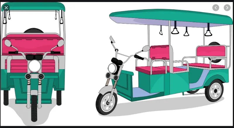
Electric rickshaws (also known as electric tuk-tuks or e-rickshaws or toto or e-tricycles) have been becoming more popular in some cities since 2008 as an alternative to the auto-rickshaws and pulled rickshaws because of their low fuel cost, and less human effort compared to pulled rickshaws. They are being widely accepted as an alternative to petrol, diesel, CNG auto-rickshaws. They are three-wheelers powered by an Electric motor ranging from 650 to 1400 Watts. They are mostly manufactured in India and China.
Design and Construction:
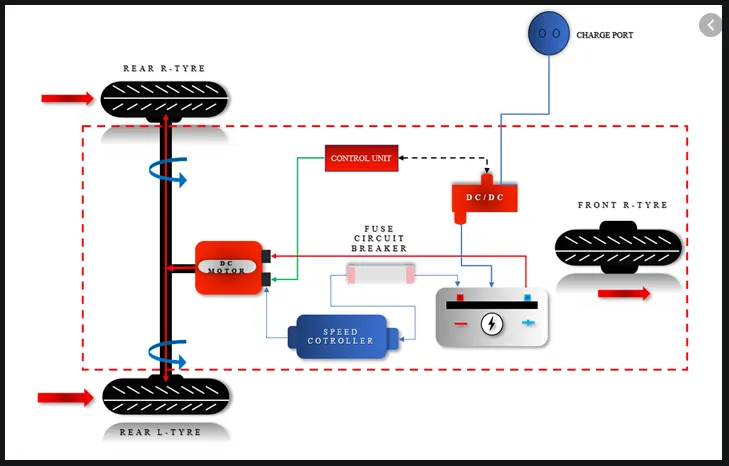
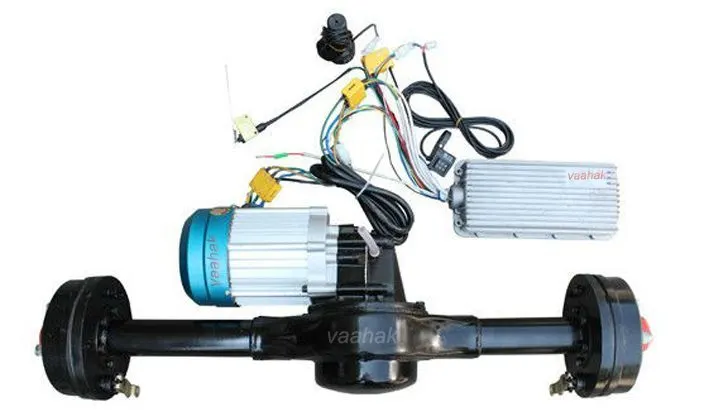
These rickshaws have an M.S(Mild Steel) tubular chassis, consisting of three wheels with a differential mechanism at the rear wheels. The motor is a brushless DC motor manufactured mostly in India and China. The electrical system used in the Indian version is 48V and in Bangladesh is 60V. The body design from the most popular Chinese version is of very thin iron or aluminum sheets. Vehicles made in fiber are also popular because of their strength and durability, resulting in low maintenance, especially in India. The body design is varied from load carriers, passenger vehicles with no roof, to full body with windshield for drivers comfort. It consists of a controller unit. They are sold on the basis of voltage supplied and current output, also the number of MOSFET (metal oxide field-effect transistors) used. The battery used is mostly a lead-acid battery with life of 6–12 months. Deep cycle batteries designed for electric vehicles are rarely used.
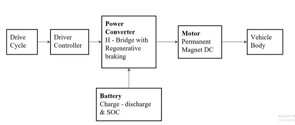
we divided our model into some part as below:
1) Drive cycle and Driver controller.
2) Power converter
3) Battery System and SOC.
4)Motor
5) Vehicle body
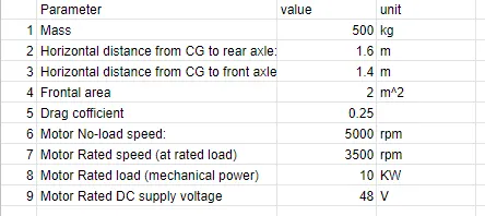
Excel sheet of all input and assumed data
Simulink Model:
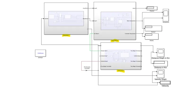
Simulink model consist of three subsytem.
Subsytem 1:
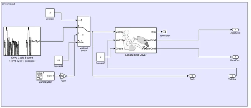
Major blocks in the subsystem are :-
- Longitudnal driver
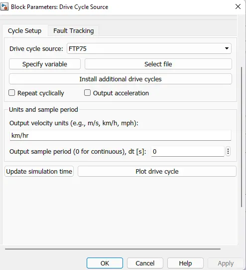
- Drive cycle source
- Signal builder
- Multiport switch
Longitudnal driver :
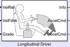
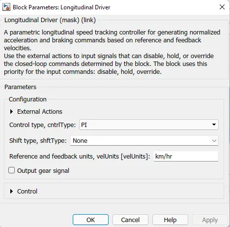
A parametric longitudinal speed tracking controller for generating normalized acceleration and braking commands based on reference and feedback velocities.
for this model our reference velocity is velocity from either from drive cycle source signal builder block or a constant as per needed and feedback velocity is from vehicle body block.
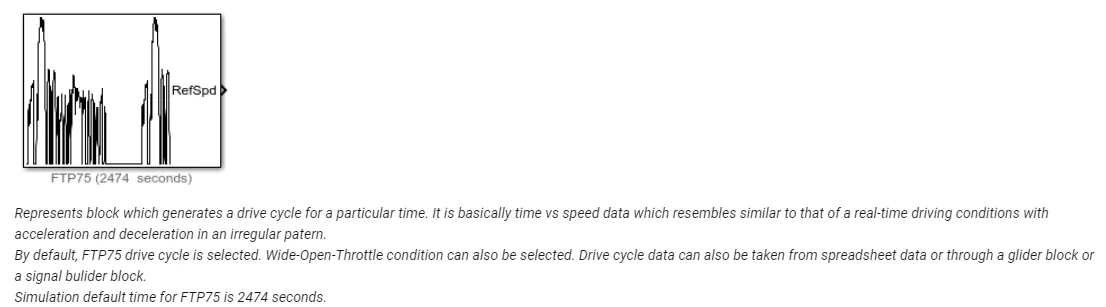
- Drive cycle source block
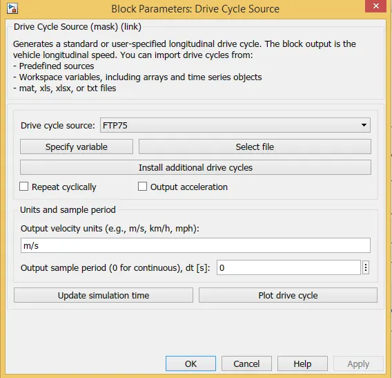
This block generates a standard or user-specified longitudinal drive cycle. The block output is the vehicle longitudinal speed.
You can import drive cycles from:
- Predefined sources
- Workspace variables, including arrays and time series objects
- mat, xls, xlsx, or txt files
Use the fault tracking parameters to identify drive cycle faults within specified speed and time tolerances.
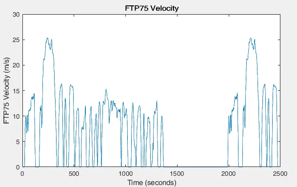
Driving cycle :- A driving cycle is a series of data points representing the speed of a vehicle versus time.
Example :- Cycle US FTP75
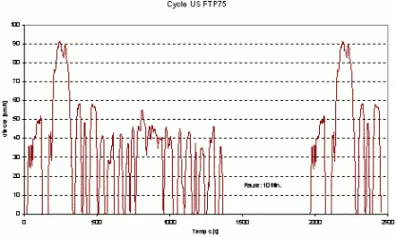
we have used FTP75 itself in this simulation.
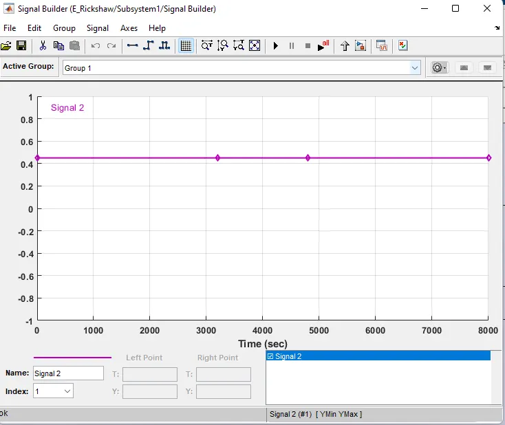
- Signal builder :
signal builder block is used along with gain block of 100.
Subsytem 2:
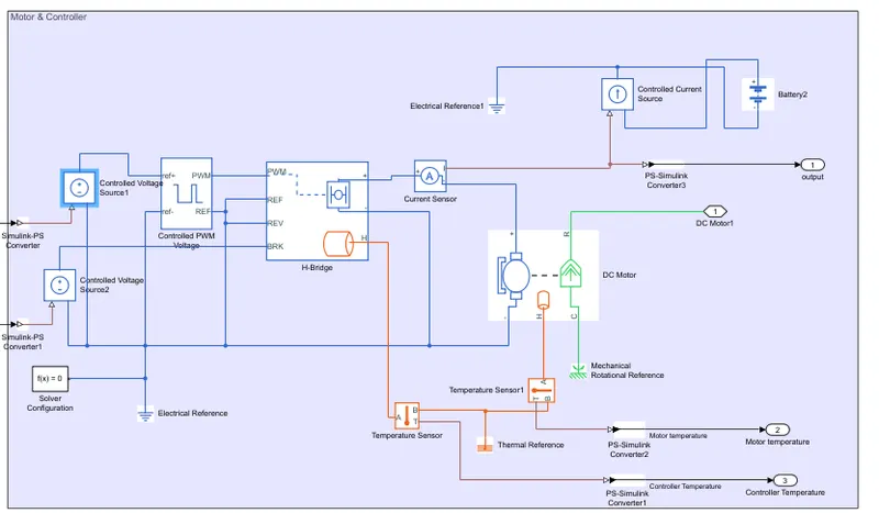
Major blocks in the subsystem are :-
- Controlled voltage source
- Controlled current source
- constant pwm source
- H -Bridge
- DC Motor
- Battery
- Temperature Sensor
Controlled voltage source :

The block represents an ideal voltage source that is powerful enough to maintain the specified voltage at its output regardless of the current passing through it. The output voltage is V = Vs, where Vs is the numerical value presented at the physical signal port.
Controlled current source
The block represents an ideal current source that is powerful enough to maintain the specified current through it regardless of the voltage across it. The output current is I = Is, where Is is the numerical value presented at the physical signal port
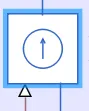
constant pwm source
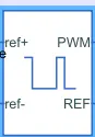
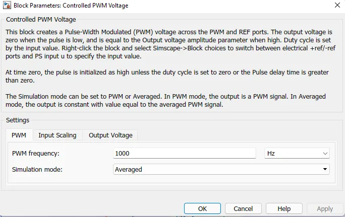
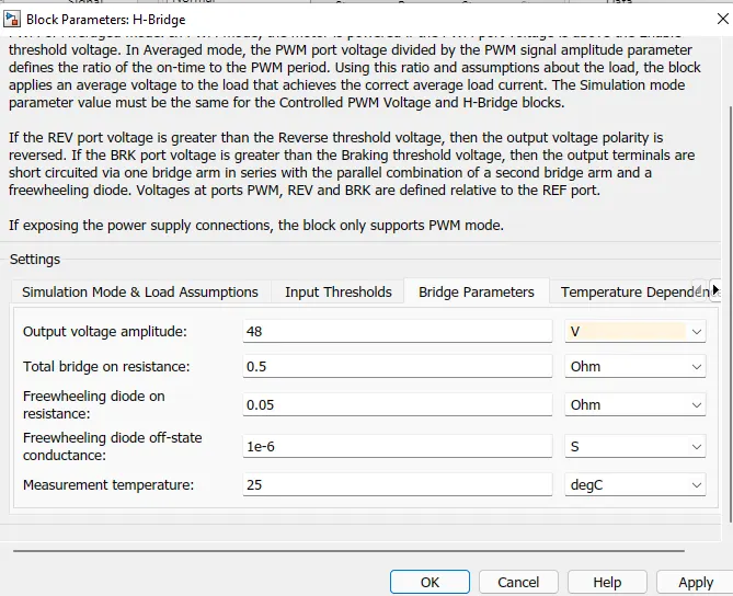
This block creates a Pulse-Width Modulated (PWM) voltage across the PWM and REF ports. The output voltage is zero when the pulse is low, and is equal to the Output voltage amplitude parameter when high. Duty cycle is set by the input value. Right-click the block and select Simscape->Block choices to switch between electrical +ref/-ref ports and PS input u to specify the input value.
H -Bridge
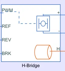
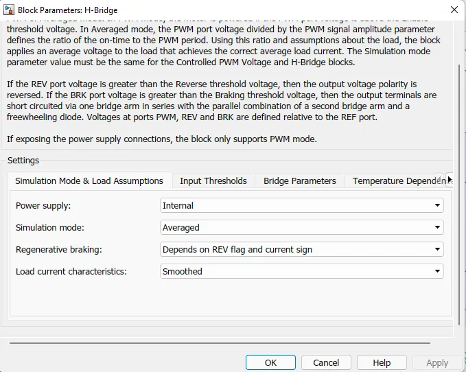
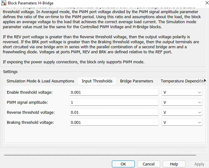
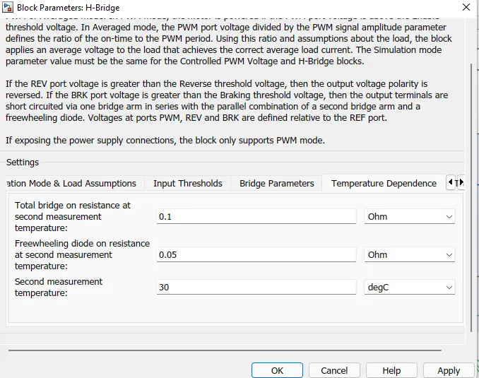
This block represents an H-bridge motor drive. The block can be driven by the Controlled PWM Voltage block in PWM or Averaged mode. In PWM mode, the motor is powered if the PWM port voltage is above the Enable threshold voltage. In Averaged mode, the PWM port voltage divided by the PWM signal amplitude parameter defines the ratio of the on-time to the PWM period. Using this ratio and assumptions about the load, the block applies an average voltage to the load that achieves the correct average load current. The Simulation mode parameter value must be the same for the Controlled PWM Voltage and H-Bridge blocks.
DC Motor
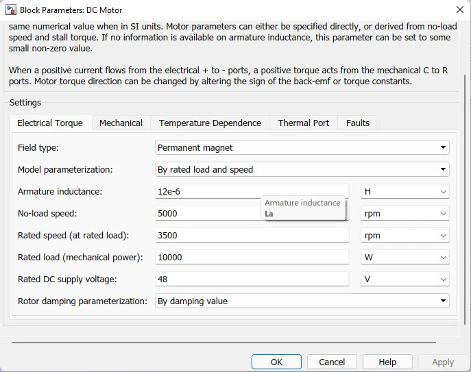
This block represents the electrical and torque characteristics of a DC motor.
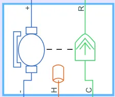
A permanent magnet (PM) motor does not have a field winding on the stator frame, instead relying on Permanent magnets to provide the magnetic field against which the rotor field interacts to produce torque.
No load speed :The no load speed is the RPM at which the DC Motor’s shaft rotate when there is no load attached to it (no torque applied to the output shaft).
Rated speed : The rated speed is the speed at which the motor will first produce its maximum designed power output, and “maximum speed,” the fastest the motor can spin while producing that same amount of power.
DC motor with controller:
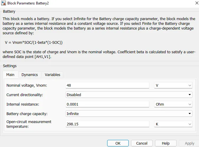
Battery
This block models a battery.We select Infinite for the Battery charge capacity parameter, the block models the battery as a series internal resistance and a constant voltage source.

- Thermal Port:
-
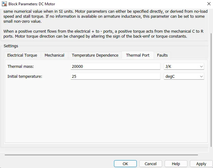
The block has an optional thermal port, hidden by default. To expose the thermal port, right-click the block in your model, and then from the context menu select Simscape > Block choices > Show thermal port. This action displays the thermal port H on the block icon, and exposes the Temperature Dependence and Thermal Port parameters.
Use the thermal port to simulate the effects of copper resistance losses that convert electrical power to heat. For more information on using thermal ports and on the Temperature Dependence and Thermal Port parameter.
- Temperature Sensor:
-
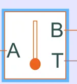
This block measures temperature in a thermal network. There is no heat flow through the sensor. The physical signal port T reports the temperature difference across the sensor. The measurement is positive when the temperature at port A is greater than the temperature at port B.
Subsytem 3:-
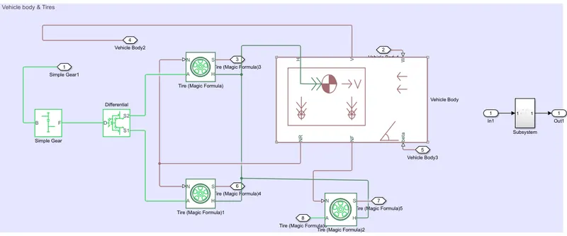
Major blocks in the subsystem are :-
- Simple gear
- Diffrential
- Tire
- Vehicle body
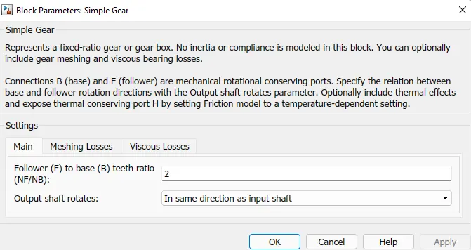
Simple gear
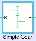
Represents a fixed-ratio gear or gear box. No inertia or compliance is modeled in this block. You can optionally include gear meshing and viscous bearing losses
Diffrential
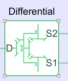
The differential is a system of gears that allows different drive wheels (the wheels to which power is delivered from the engine) on the same axle to rotate at different speeds, such as when the car is turning.
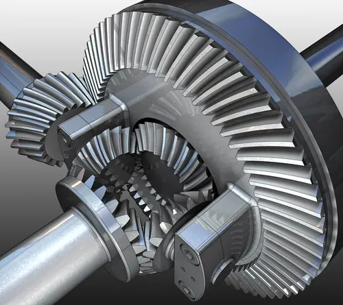
This block represents a differential which is arranged as a planetary bevel gear train equipped with an additional bevel gear transmission between the driveshaft and the carrier. The pinion gear of this transmission is attached to the driveshaft while the large bevel crown gear is affixed to the carrier. Compliance is not modeled in this block. Optionally include inertia and losses from gear meshing and viscous bearing friction.
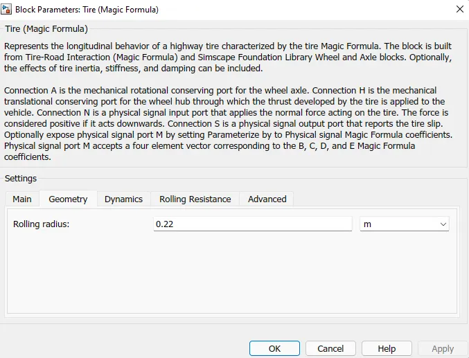
Tire
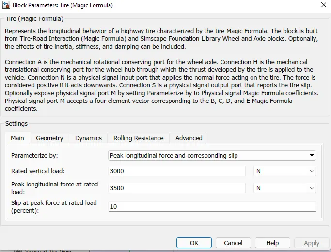
This block represents the longitudinal behavior of a highway tire characterized by the tire Magic Formula.
The block is built from Tire-Road Interaction (Magic Formula) and Simscape Foundation Library Wheel and Axle blocks. Optionally, the effects of tire inertia, stiffness, and damping can be included
vertical load (Fz)
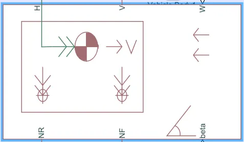
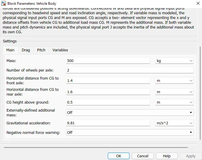
Vehicle body :
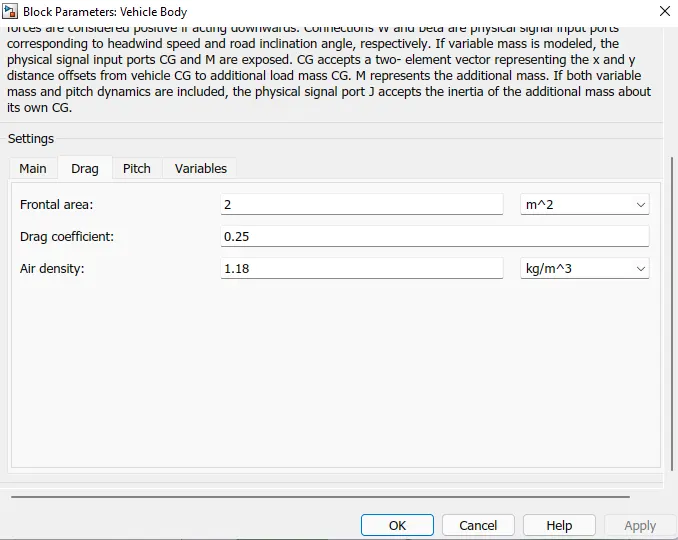
Represents a two-axle vehicle body in longitudinal motion. The block accounts for body mass, aerodynamic drag, road incline, and weight distribution between axles due to acceleration and road profile. The vehicle can have the same or a different number of wheels on each axle. Optionally include pitch and suspension dynamics or additional variable mass and inertia. The vehicle does not move vertically relative to the ground.
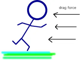
Drag force -
Drag force is the resistance force of a fluid. This force applies acting opposite towards the motion of the object which is moving submerge in a certain fluid. Thus Drag Force is defined as the force which resists the motion of a body with fluid.
Result :
1) Using FTP 75 drive cycle.
Simulation Time: 2474 seconds
Distance Travelled: 5.5 m/s or 20 Km
The reference velocity of vehicle (Yellow curve) almost matches with the actual velocity of vehicle (Blue Curve) with the max speed of around 25 m/s as shown in fig.1.1. This small deviation is due to the inertial effect & its control parameter.
Fig.1.2. shows the detailed view of how the close the reference speed matches the actual speed from 100-500 seconds
Fig.1.3. shows the variation in the current. As the speed increases more current is drawn from the battery. The current curve reaches the negative value during regenerative braking which draws current for the Battery to charge.
Fig.1.4. shows the SOC of the Battery. For 2474 seconds the Battery reaches from 100 % to 60 %. Hence 40% Battery is consumed for the vehicle to travel for around 5.5 m/s or 20 Km. Also there is rise in SOC curve at some points due to the regenerative braking that charges the Battery.
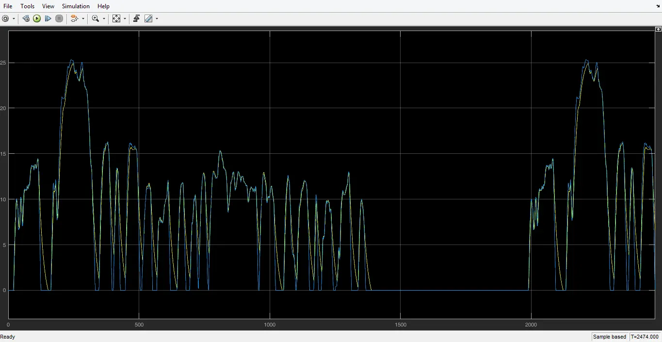
Fig.1.1. Speed Curve
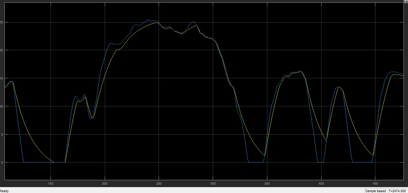
Fig.1.2. Speed Curve (Zoomed View)
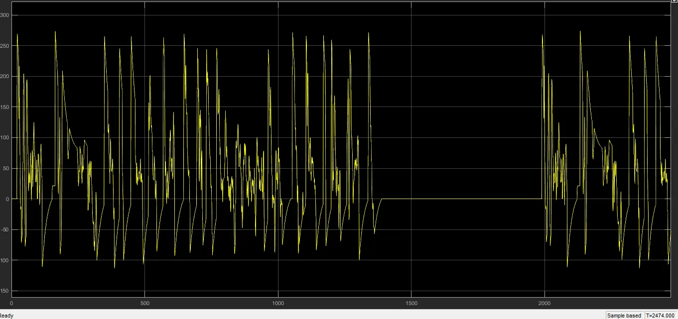
Fig.1.3. Current Curve
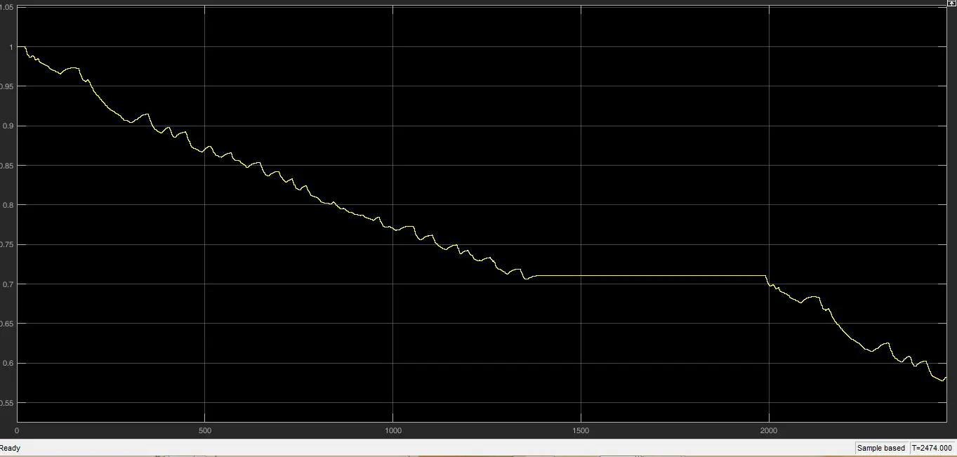
Fig.1.4. SOC of Battery
2) Wide Open Throttle by using signal builder block
Simulation time : 8005 seconds
Speed after adding gain of 100 : 45 kmph
Distance travelled
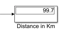
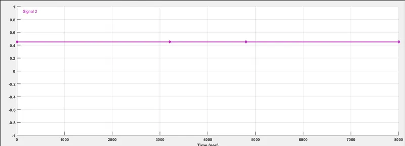
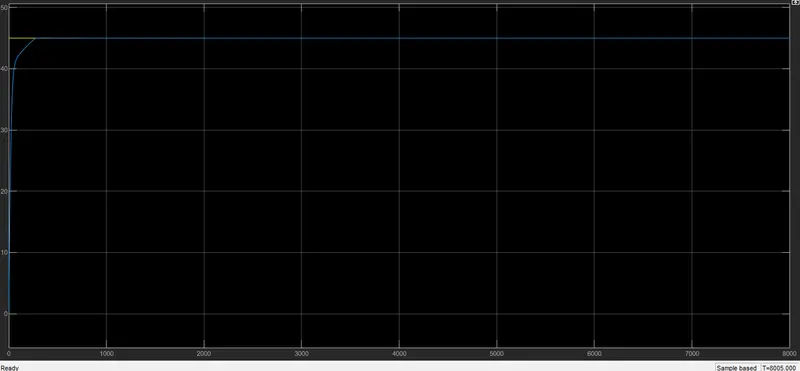
In WOT Condition we could see that the reference speed curve match with the Vehicle speed around 290 sec.
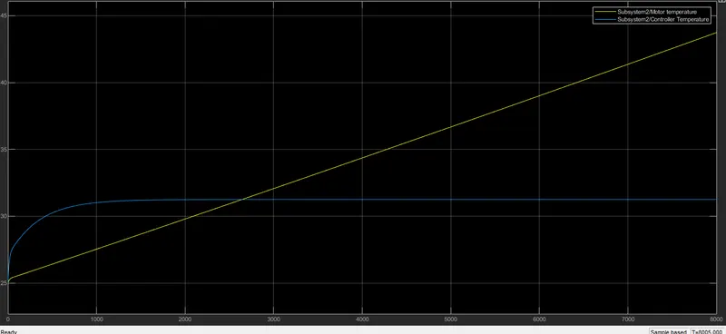
Motor tempereture at the end of simulation reached 43.7 degree Celcius.
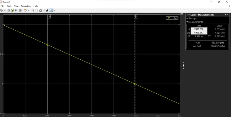
In The SOC of the battery has reached 0 in around 5955 seconds.
Conclusion
As per the Motor specification, Type of controller, Vehicle Parameters & Battery used we could see that the reference speed almost matches with the vehicle speed for the drive cycle FTP 75 and WOT condition.