Final Project: Electric Rickshaw modelling

AIM:

Create a detailed MATLAB model of an electric rickshaw (three wheel passenger vehicle) as per details below:

• Rear wheels driven by PM brushed type motor
• Assume efficiency points of motor controller and motor
• Make an excel sheet of all input and assumed data

Results: For any three standard driving cycles show energy consumption, temperature rise of motor and controller for 100 kms, constant speed driving at 45 kmph

OBJECTIVE:

• Make a model with the appropriate blocks
• Ensure with the inputs of each blocks involved in the model
• Check the efficiency points for each cases
• Summarize the data in a tabular format through excel

1. Create a detailed MATLAB model of an electric rickshaw (three wheel passenger vehicle) as per given details

Following will shows the detailed information of the electric rickshaw with a matlab model,

Introduction of Electric Rickshaw:

• Electric rickshaws (also known as electric tuk-tuks or e-rickshaws or toto or e-tricycles) have been becoming more popular in some cities
• The electric rickshaw has been global since 1940's from the time of post era. But, its utilization and popularity have actually come into prominence since last 10-12 years
• Actually, the concept of tricycles with fuel run emerged at that time, after that the auto rickshaws has dominated the market

• It is only in the year 2008 that battery operated rickshaw gain much importance worldwide because of their low fuel cost and less human effort compared to pulled rickshaws
• They are being widely accepted as an alternative to petrol/diesel/CNG auto rickshaws. They are three-wheelers powered by an electric motor ranging from 650 to 1400 Watts
• They are mostly manufactured in India and China. Battery-run rickshaws could be a low-emitter complementary transport for the low-income people, who suffer most from a lack of transport facility, if introduced in a systematic manner according to experts

Construction of E-Rickshaw:

• No doubt that battery operated vehicle is robust and strong enough. Also, it is ensured that this vehicle provides all the facility for the comfort of every passenger
• No doubt there are a hell lot of rickshaw spare parts required for the construction of "e-rickshaw". Also, the vehicle is crafted with the best quality of metal and fiber glass
• Among the other materials, an open frame is used for the construction of these e-rickshaws. The rickshaw is no doubt cost-effective because it is battery operated as well as consumes less energy
• The 3 wheeler e- rickshaw is definitely the best substitute for fuel driven vehicles and efficient when comes to battery power
• Also, there is no emission of harmful pollutants from this vehicle so it helps to increase the durability and strengthens the vehicle
• The materials which are used in constructing the vehicle such as fibre-glasses help it to make the vehicle more efficient. Also, this vehicle is absolutely perfect to cover the short distance as well as carry small loads

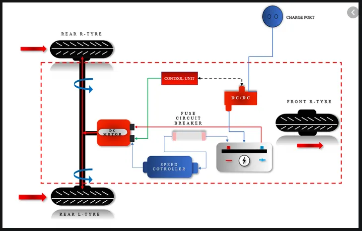
Working Principle:

• The body weight of the E- rickshaw is extremely light and because of that durability of the battery does not get decreased
• The main elements that actually drive the electric rickshaw are a motor, controller, harness and most importantly its throttle
• To get the best service and to increase the benefits from this vehicle these elements are essential
• The motor of the battery generally varies from 650W to 1250W while according to the rules the unit should not increase 650W
• Moreover, these E-rickshaws constitute of leaf spring suspension. The power supplies at the rate of 48 V which can also be controlled by a specific controller
• It is essential that manufacturers use the superior quality battery to get the best performance and takes care that the batteries don't get overheated very fast
• The best part of this rickshaw is that they need minimal maintenance. Although it is important that at regular intervals the vehicle must be taken to the service centres
• Any misuse with the vehicle might affect the entire system. Also, wrong adjustments with the brakes might also affect the motor and other essential elements. If this happens then not only it will severely affect the vehicle but also decrease the mileage

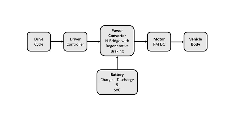
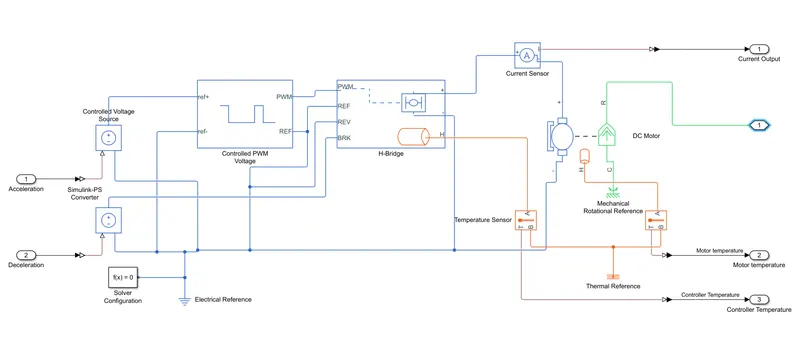
E-Rickshaw Simulink Model:

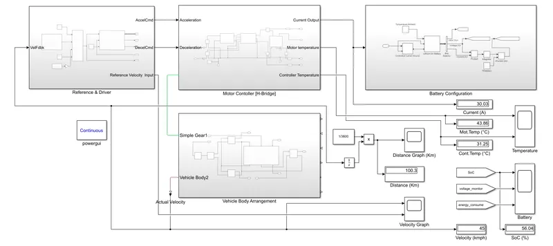
Note: The above simulink model's file has attached for the reference

Following will explain as detailed for the each subsystems,

1. Reference Inputs Setup:

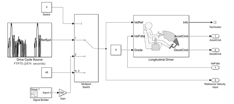
FTP75:

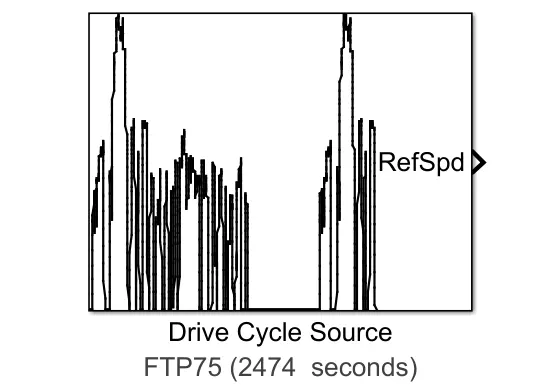
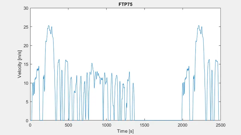
• The reference inputs for the e-rickshaw model are FTP75 and WOT were used. Drive cycles from predefined sources. By default, the block includes the FTP–75 drive cycle

WOT:

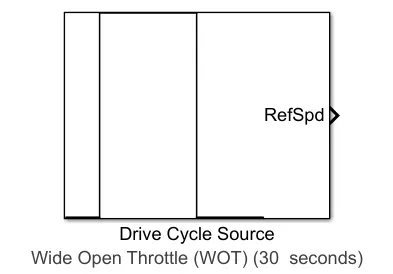
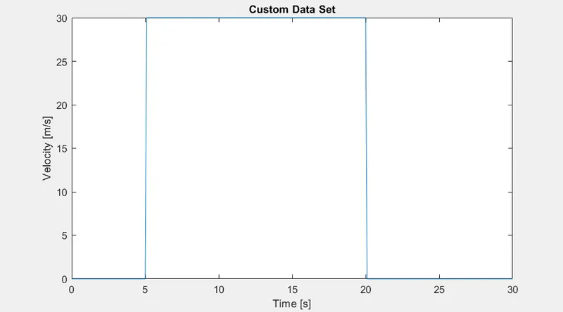
• Wide open throttle (WOT) parameters, including initial and nominal reference speed, deceleration start time and final reference speed

Signal Builder:

• The Signal Builder block allows you to create interchangeable groups of piecewise linear signal sources and use them in a model
• We can quickly switch the signal groups into and out of a model to facilitate testing. In the Signal Builder window, create signals and define the output waveforms

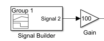
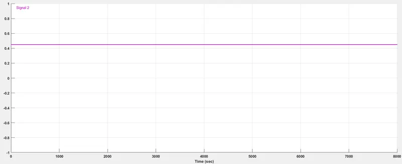
• The feeded value is 0.45 for the entire run time and it multiplied with the "gain block" has the value of 100

Multiport Switch:

• The multiport switch block has used to switch the output signal based on the control signal for the velocity reference in the longitudinal driver block

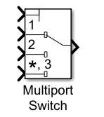
• The Multiport Switch block determines which of several inputs to the block passes to the output. The block bases this decision on the value of the first input
• The first input is the control input and the remaining inputs are the data inputs. The value of the control input determines which data input passes to the output

Longitudinal Driver:

• Here I have used this block only with the default values like PI control type which is proportional-integral (PI) control with tracking windup and feed-forward gains

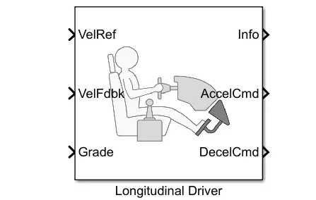
• The Longitudinal Driver block implements a longitudinal speed-tracking controller. Based on reference and feedback velocities, the block generates normalized acceleration and braking commands that can vary from 0 through 1
• And also can use the block to model the dynamic response of a driver or to generate the commands necessary to track a longitudinal drive cycle

2. Motor Controller:

Controlled PWM Voltage:

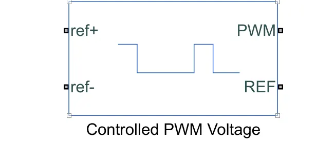
• The Controlled PWM Voltage block represents a pulse-width modulated (PWM) voltage source. The block has two modeling variants, accessible by right-clicking the block in your block diagram and then selecting the appropriate option from the context menu, under Simscape > Block choices:
• 1. Electrical input ports — The block calculates the duty cycle based on the reference voltage across its ref+ and ref- ports. This modeling variant is the default
• 2. PS input — Specify the duty cycle value directly by using an input physical signal port
• We going to use the default option of Electrical input ports

H-Bridge:

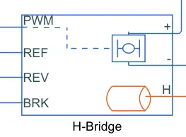
• For make to show the thermal port, follow the instructions,

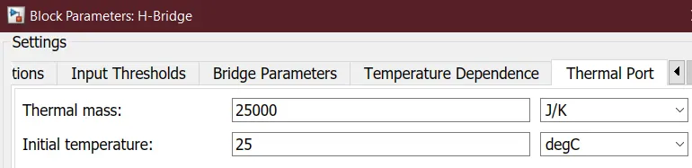
• The heat generated by the bridge on-resistance and freewheeling diodes is added to the thermal port. The thermal port has an associated thermal mass and initial temperature that you can set from the Thermal Port parameters
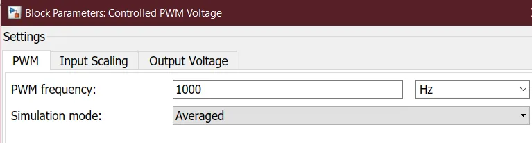
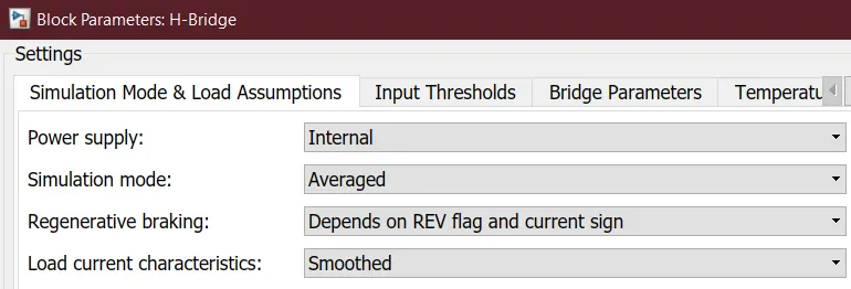
• The H-Bridge block represents an H-bridge motor driver. This block has the same simulation mode options like controlled PWM voltage, we have to choose same as averaged
• It speed up simulations when driving the H-Bridge block with a Controlled PWM Voltage block. You must also set the Simulation mode parameter of the Controlled PWM Voltage block to Averaged mode
• This applies the average of the demanded PWM voltage to the motor. The accuracy of the Averaged mode simulation results relies on the validity of your assumption about the load current
• Smoothed — Assumes that the current is practically continuous due to load inductance. This option is the default
• If you specify that the current is Unsmoothed or discontinuous, then the accuracy also depends on the values you provide for load resistance and inductance being representative
• This mode also makes some simplifying assumptions about the underlying equations for the case when current is discontinuous
• For typical motor and bridge parameters, accuracy should be within a few percent. To verify Averaged mode accuracy, run the simulation using the PWM mode and compare the results to those obtained from using the Averaged mode
• If you are linearizing your model, set the Simulation mode parameter to Averaged and ensure that you have specified the operating point correctly
• You can only linearize the H-Bridge block for duty cycles that are greater than zero and less than the PWM signal amplitude
• If you need to linearize around zero duty cycle, and if your controller always uses regenerative braking mode, set the Regenerative braking parameter to Always enabled (suitable for linearization)

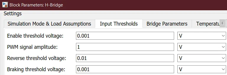
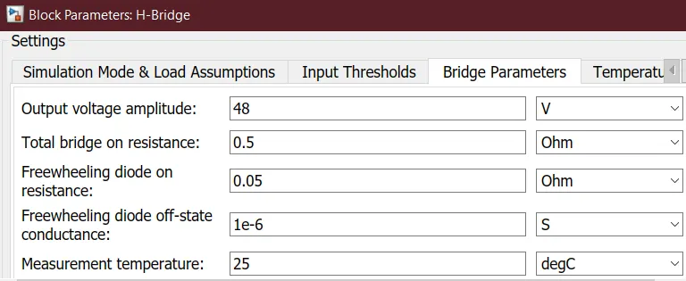
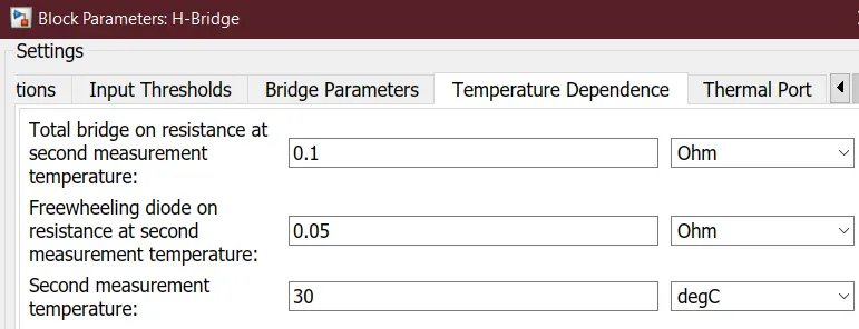
Following parameters are the inputs were used in the H-bridge block,

DC Motor:

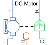
• For make to show the thermal port, follow the instructions,

• DC Motor model using the physical modeling blocks of the Simscape extension to Simulink. The blocks in the Simscape library represent actual physical components
• Therefore, complex multi-domain models can be built without the need to build mathematical equations from physical principles by applying Newton's laws and Kirchoff's laws

Following parameters are the inputs were used in the DC motor block,

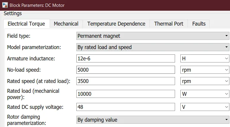
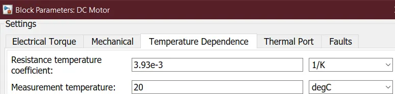
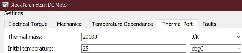
• Remaining inputs for the DC motor block are remains as default

Supporting Blocks:

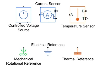
Those are controlled voltage source, current sensor, temperature sensor and references: mechanical rotational, electrical and thermal

3. Vehicle Body Arrangement:

Vehicle Body:

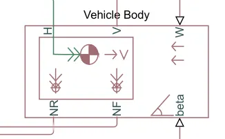
• Connection H is the mechanical translational conserving port associated with the horizontal motion of the vehicle body. The resulting traction motion developed by tires should be connected to this port
• Connections V, NF, NR are physical signal output ports for vehicle velocity and front and rear normal wheel forces, respectively. Wheel forces are considered positive if acting downwards
• Connections W and beta are physical signal input ports corresponding to headwind speed and road inclination angle as respectively
• The Vehicle Body block represents a two-axle vehicle body in longitudinal motion. The vehicle can have the same or a different number of wheels on each axle
• In here based on the rickshaw model, single wheel on the front axle and two wheels on the rear axle. The vehicle wheels are assumed identical in size. The vehicle can also have a center of gravity (CG) that is at or below the plane of travel
• The block accounts for body mass, aerodynamic drag, road incline and weight distribution between axles due to acceleration and road profile
• Optionally include pitch and suspension dynamics. The vehicle does not move vertically relative to the ground
• The block has an option to include an externally-defined mass and an externally-defined inertia. The mass, inertia and center of gravity of the vehicle body can vary over the course of simulation in response to system changes

Tire (Magic Formula):

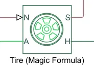
• The Tire (Magic Formula) block models a tire with longitudinal behavior given by the magic formula, an empirical equation based on four fitting coefficients
• The block can model tire dynamics under constant or variable pavement conditions
• The longitudinal direction of the tire is the same as its direction of motion as it rolls on pavement. This block is a structural component based on the Tire-Road Interaction (Magic Formula) block
• To increase the fidelity of the tire model, you can specify properties such as tire compliance, inertia, and rolling resistance
• However, these properties increase the complexity of the tire model and can slow down simulation. Consider ignoring tire compliance and inertia if simulating the model in real time or if preparing the model for hardware-in-the-loop (HIL) simulation

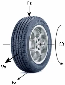
• The above image shows the forces acting on the tire. The Tire (Magic Formula) block models the tire as a rigid wheel-tire combination in contact with the road and subject to slip
• When torque is applied to the wheel axle, the tire pushes on the ground (while subject to contact friction) and transfers the resulting reaction as a force back on the wheel
• This action pushes the wheel forward or backward. If you include the optional tire compliance, the tire also flexibly deforms under load

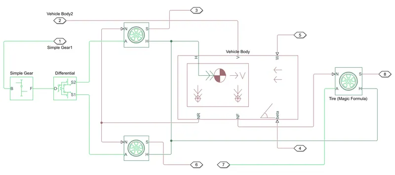
• Here the tire slips were terminated with the PS terminator for both front and back tyres as respectively

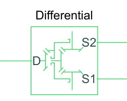
• The Differential block represents a gear mechanism that allows the driven shafts to spin at different speeds
• Differentials are common in automobiles, where they enable the various wheels to spin at different speeds while cornering
• Ports D, S1, and S2 represent the longitudinal driveshaft and the sun gear shafts of the differential as respectively. Any one of the shafts can drive the other two
• To increase the fidelity of the gear model, specify properties such as gear inertia, meshing losses and viscous losses. By default, gear inertia and viscous losses are assumed to be negligible
• The block enables you to specify the inertias of the gear carrier and internal planet gears. To model the inertias of the outer gears, connect simscape "inertia blocks" to ports D, S1, and S2

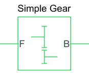
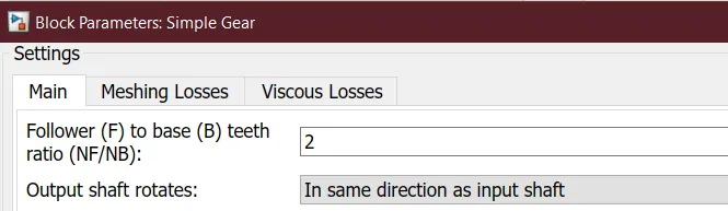
• The Simple Gear block represents a gearbox that constrains the connected driveline axes of the base gear (B) and the follower gear (F) to co-rotate with a fixed ratio that you specify
• we can choose whether the follower axis rotates in the same or opposite direction as the base axis. If they rotate in the same direction, the angular velocity of the follower (ωF) and the angular velocity of the base (ωB) have the same sign. If they rotate in opposite directions, ωF and ωB have opposite signs

4. Battery Configuration:

Battery:

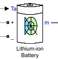
• The Battery block implements a generic dynamic model that represents most popular types of rechargeable batteries
• Implements a generic battery model for most popular battery types. Temperature and aging (due to cycling) effects can be specified for Lithium-Ion battery type

Charge and Discharge Characteristics:

• The circuit parameters can be modified to represent a specific battery type and its discharge characteristics. A typical discharge curve consists of three sections

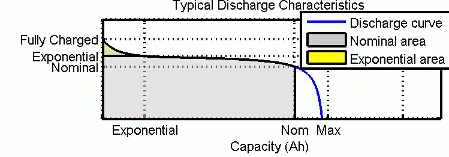
• The first section represents the exponential voltage drop when the battery is charged. The width of the drop depends on the battery type
• The second section represents the charge that can be extracted from the battery until the voltage drops below the battery nominal voltage. Finally, the third section represents the total discharge of the battery, when the voltage drops rapidly
• When the battery current is negative, the battery recharges, following a charge characteristic:

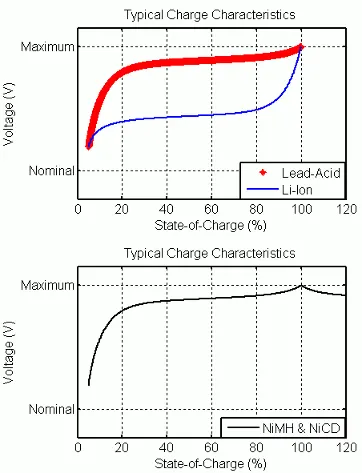
• The model parameters are derived from the discharge characteristics. The discharging and charging characteristics are assumed to be the same
• The exponential transfer function represents the hysteresis phenomenon for the lead-acid, nickel-cadmium (NiCD), and nickel-metal hydride (NiMH) batteries during the charge and discharge cycles
• The exponential voltage increases when a battery is charging, regardless of the battery's state of charge. When the battery is discharging, the exponential voltage decreases immediately
• The state of charge (SOC) for a battery is a measure of battery's charge, expressed as a percent of the full charge. The depth of discharge (DOD) is the numerical compliment of the SOC, such that DOD = 100% - SOC.

For example, if the SOC is:

1. 100% - The battery is fully charged and the DOD is 0%
2. 75% - The battery is 3/4 charged and the DOD is 25%
3. 50% - The battery is 1/2 charged and the DOD is 50%
4. 0% - The battery is has 0 charge and the DOD is 100%

Model Validation:

• Experimental validation of the model shows a maximum error of 5% (when SOC is between 10% and 100%) for the charge (when the current is 0 through 2 C) and discharge (when the current is 0 through 5 C) dynamics

Controlled Current Source:

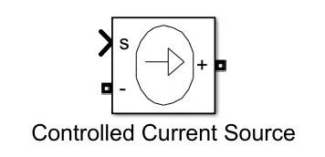
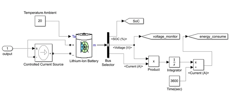
• It converts the simulink input signal into an equivalent current source. The generated current is driven by the input signal of the block
• Motor current sensor has converted and connect with the source (s)
• Select current in the measurement option on controlled current source
• Connect (+) terminal in the (-) terminal of the battery
• Connect (-) terminal in the (+) terminal of the battery
• Connect constant value of 20 temperature ambient in the Ta of the battery

Bus Selector:

• This block accepts a bus as input which can be created from a Bus Creator, Bus Selector or a block that defines its output using a bus object
• The left listbox shows the elements in the input bus. Use the Select button to select the output elements
• The right listbox shows the selections. Use the Up, Down, or Remove button to reorder the selections

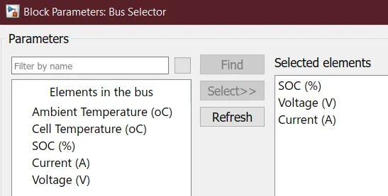
• Connect SoC, voltage with goto blocks as directly to show the output in the main scope
• Make the current output to product with the voltage value to find the energy consumption
• And use the powergui block to set the simulation type as continuous

5. Total Distance Calculation:

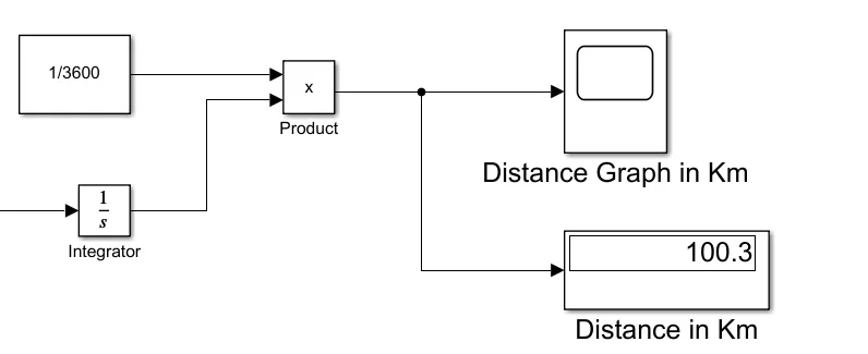
• The total distance travelled (100kms) has calculated by the some bas calculation with the input of velocity feedback reference
• The value it has passed to the integrator to outputs the value of the integral of its input signal with respect to time (continuous-time)
• And it's output has multiplied with the constant value (1/3600) by using the product block has finally passed to the scope and display blocks to show the final output

Note:

`Time(seconds)= (Distance(kms))/(Speed (kmph))`

`=100/45*3600`

`=8000`

• Based on some power loss, 50 seconds were added in the total run time for achieve the distance of 100kms

Simulation stop time: 8050 seconds

EXCELSHEET OF ALL INPUTs & ASSUMED DATA:

E-RICKSHAW OVERALL INPUTS
S.No	PARAMETERS	VALUES	UNIITS
Controlled PWM Voltage
1	PWM frequency	1000	Hz
2	Simulation mode:	Averaged
H-Bridge With Thermal Port
Simulation Mode & Load Assumptions
3	Simulation mode:	Averaged
Input Thresholds
4	Enable threshold voltage	0.001	V
5	PWM signal amplitude	1	V
6	Reverse threshold voltage	0.01	V
7	Braking threshold voltage	0.001	V
Bridge Parameters
8	Output voltage amplitude	48	V
9	Total bridge on resistance	0.5	Ohm
10	Measurement temperature	25	°C
Temperature Dependence
11	Second measurement temperature	30	°C
Thermal Port
12	Thermal mass	25000	J/K
13	Initial temperature	25	°C
DC Motor
Electrical Torque
14	Model parameterization	By rated load & speed
15	No-load speed	5000	rpm
16	Rated speed (at rated load)	3500	rpm
17	Rated load (mechanical power)	10000	W
18	Rated DC supply voltage	48	V
Temperature Dependence
19	Measurement temperature	20	°C
Thermal Port
20	Thermal mass	20000	J/K
Vehicle Body
Main Setting
21	Mass	500	kg
Drag
22	Frontal area	2	m/s^2
23	Drag coefficient	0.25	No Unit
Frontal And Rear Tire
Geometry
24	Rolling radius	0.22	m
Rolling Resistance
25	Rolling resistance	ON
Lithium-Ion Battery
26	Nominal voltage	48	V
27	Rated capacity	153.54	Ah

Note: The above overall inputs tabulation has described in an excel sheet and the file has attached for the reference

RESULTS:

1. Motor Temperature & Controller Temperature

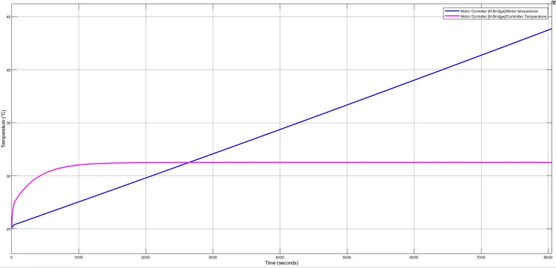
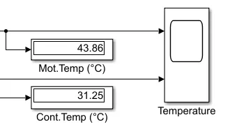
• From the reading of motor and controller temperature, the vehicle has travelled for 100 kms distance on 2.22 hrs (8000 secs), so that temperaure has raised upto 43.86°C for motor and 31.25°C for controller as respectively

2. Velocity Graph:

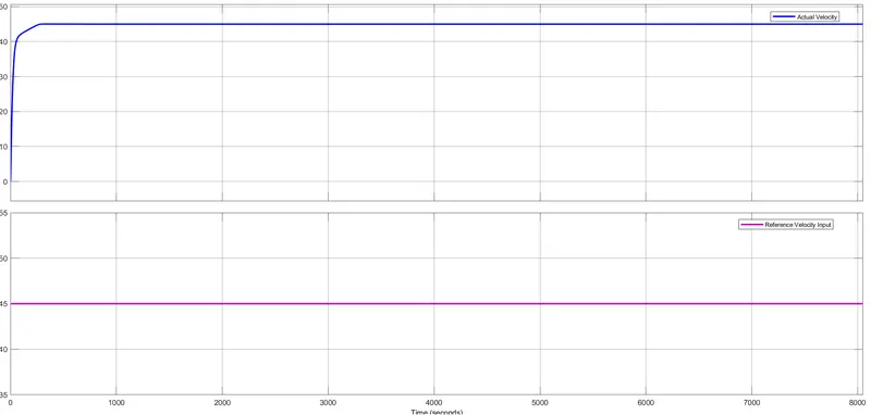
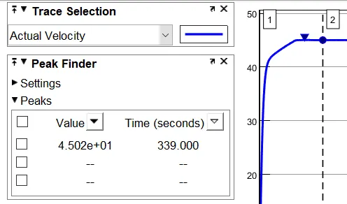
• From the reading of velocity graph, the actual velocity has reached to it's position as per the reference input velocity at it's 339th seconds

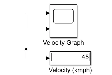
• For the one more clarification, the final velocity output has shown in the display block,

3. Battery Parameters

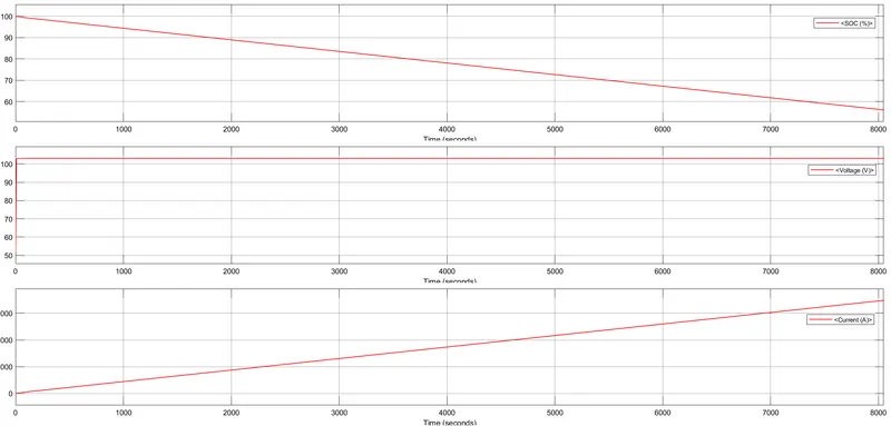
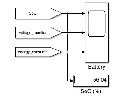
• From the reading of battery parameters on the overall battery usage by the vehicle, (DOD% - SoC%) the state of charge has remains 56.04%
• And the voltage and current has passed upto the end was 103.1V and 6953Amps from the battery

REFERENCES:

Modeling of Electric Vehicles using MATLAB & Simulink-

• Part-1: https://www.youtube.com/watch?v=tM9Akdo8QeA&list=RDCMUCc6AKorV1iA6CmM3yT2CKjA&index=2
• Part-2: https://www.youtube.com/watch?v=xmdUFEfiAKk&list=RDCMUCc6AKorV1iA6CmM3yT2CKjA&index=3

CONCLUSION:

• The working concept of the PWM controller, H-bridge and DC motor were understood
• The simulink connections for the major subsystems of the electric vehicle has learned well
• Feeded inputs on the simulink model were detailed in the spreadsheet for the references
• Acquired a knowledge of the control system of the electric vehicle through the simulink