Final Project: Electric Rickshaw modelling

AIM: To model an Electric Rickshaw with suitable Blocks in MATLAB and Simulink and analyse the results.

OBJECTIVES:

• Make sure the rear wheels of the rickshaw should be power by PM brushed type motor only.
• We can assume the efficiency points of Motor and Motor Controller.
• Analyse the results for any three-driving cycle and show the energy consumption, temperature rise in motor and controller for 100km constant speed driving at 45 kmph.

Create a detailed MATLAB model of an electric rickshaw (three-wheel passenger vehicle) as per details below:

Rear wheels driven by PM brushed type motor

Assume efficiency points of motor controller and motor

Make an excel sheet of all input and assumed data

Results: For any three standard driving cycles show energy consumption, temperature rise of motor and controller for 100 km constant speed driving at 45 kmph.

Introduction

Electric Rickshaws are eco-friendly battery-operated three-wheelers that have a better economy and lower operational cum maintenance costs. These e-rickshaws does not emit toxic pollutants into the air during operation and hence, does not have any tailpipe. These vehicles have gained popularity amongst Indian rickshaw drivers and commuters.

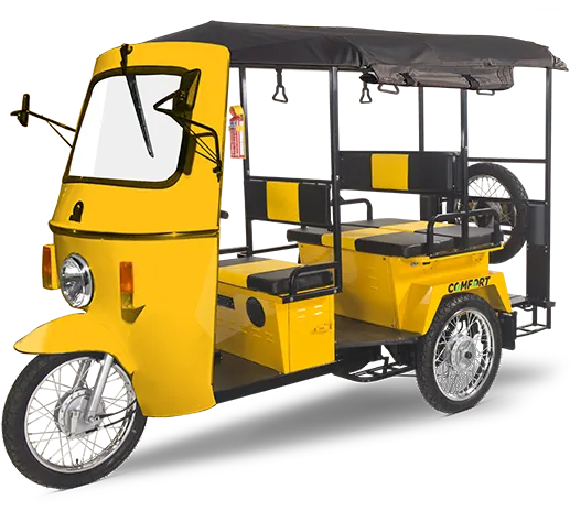
There are numerous players in India who are involved in the assembly of electric rickshaws. Most of these vehicles are assembled using sub-standard Chinese parts, which compromises the quality and performance of the vehicles. We, at GEMEV use premium quality components and raw materials to manufacture our vehicles. As a result, our products are more durable and give superior performance.

Schematic Diagram

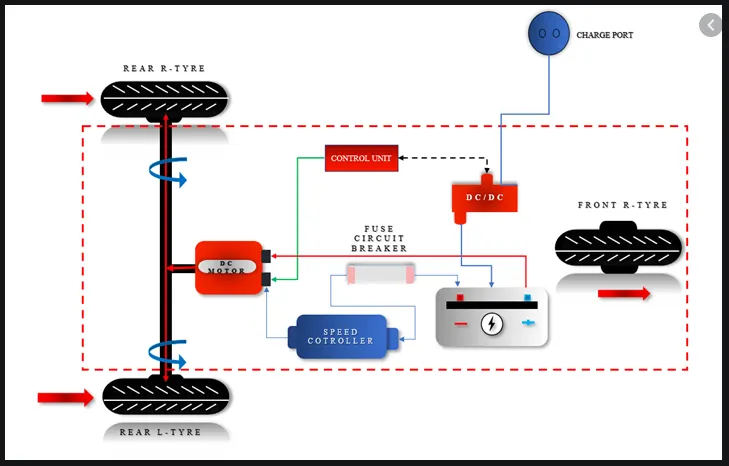
Working of Electric Rickshaw

E Rickshaw in India are built over tubular chassis, the body is kept light in weight to increase the life and performance of the battery. The main electronic components which make the powertrain are motor, controller, harness, batteries and the throttle. Any mismatch among any of these components is undesirable and may compromise vehicle performance.

The chassis is the main part which ensures drive quality and safety of the vehicle. It is made of mild steel. These days, most of the locally-made chassis are often built without proper design, leading to an imbalance in the drive, and often causing the vehicle to pivot or topple very easily. The chassis manufactured by a professional E Rickshaw Manufacturer is robust as the design adheres to all quality / technical parameters, which are often ignored by others. The chassis, if inaccurately made, will have handling problems, will be damaged easily, and corrode if not treated for resisting certain chemicals (from the battery or otherwise) or moisture.

The low weight of a body is desirable, which can be achieved with good product design, quality check, using materials such as F.R.P, aluminium, composite materials, and low-density metals. A very good alternative is F.R.P which is strong, non-conducting, cheap, lightweight, highly durable, resistant to fire, withstands weather and is easily repaired in case of damage. The body is attached to chassis by bolts, and in some cases welded, which is not recommended. The body should be built keeping in mind the quality and design which is aerodynamic and ensures driver safety. Better quality bodies last for years whereas low-quality body will last no longer than 10 to 15 months. In this case, F.R.P is extremely desirable since the life of the body runs in multiple decades. Electrical parts are recommended to be tight, use high-quality couplers to ensure proper connection and insulate connection to prevent water and moisture.

Usage of high-quality electrical components will lower resistance and heat losses and increase efficiency.

The motor power used in most e rickshaws is 650W to 1250W, the latest government norms allow it to be 650W, most of them run on 850W and higher, which adversely affects the battery life. The controller used is ~ 40A, 48V output, uses 14, 18 or 24 MOSFETs and powers all electric components.

A good quality controller must be used to increase the performance of the motor and other overheating issues. A controller should be installed with electrical brake cut off, and which usually are removed by common rickshaw mechanics in order to achieve a continuous torque or improper functioning of the brakes.

The braking system is mechanical drum brakes. Service and maintenance are required for proper vehicle functioning as the improper brake adjustments may heat up the motor and controllers and damage brake shoes. It may also reduce the mileage of the vehicle.

The batteries used in e rickshaws are lead acid as they provide low-cost alternative. They range from 80A to 120A nowadays. A larger battery with more capacity can be used, but adversely it can increase weight and reduce mileage. To prevent it, the ratio of weight and AH (measure of battery capacity) must be maintained, so we recommend to use not more than 110AH batteries as they exceed 125 kgs. Deep discharge batteries made for electric vehicles may be used depending on the customer’s preference. To maintain long life, a low amperage charger ~10 to 15A should be used, a charger with current and voltage maintained is preferred to prevent bulging and higher cycles.

Every aspect of an electric vehicle, if engineered, designed and manufactured with quality will improve battery life, vehicle life and contribute to a higher profit over time.

Note:

Important result to be obtained is the rise in temperature of motor and controller when the vehicle has travelled 100km distance at 45kmph constant speed throughout.

To do this task we need to create separate drive cycle. In this drive cycle the speed is 45kmph constant for 8000 seconds. With this given speed and time the vehicle should complete 100km.

How to calculate time (8000 seconds):

Vehicle speed = 45kmph

distance to be travelled = 100 km

Time taken to reach 100 km with constant speed of 45kmph = 100/45 = 2.22 h

converting hours to seconds = 2.22*3600 = 8000 seconds

Procedure for Modelling a Virtual Environment Electric Rickshaw in MATLAB-Simulink

• Drive cycle
• Driver Configuration
• Power Controller and Motor
• Battery (Power Source)
• Vehicle Dynamics

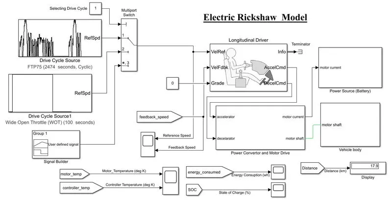
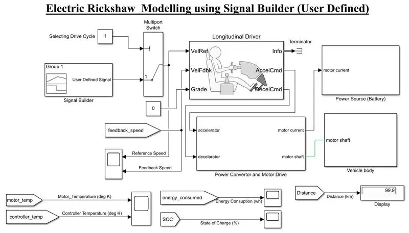
Block diagram of Electric Rickshaw:

Drive cycle:

A driving cycle is a series of data points representing the speed of a vehicle versus time. they are used in propulsion system simulations to predict performance of internal combustion engines, transmissions, electric drive systems, batteries, fuel cell systems, and similar components.

It can generate a standard or user-specified longitudinal drive cycle. The block output is the vehicle longitudinal speed. There are different types of predefined drive cycles or can add in MATLAB workspace variables, including arrays and time series objects or spreadsheets.

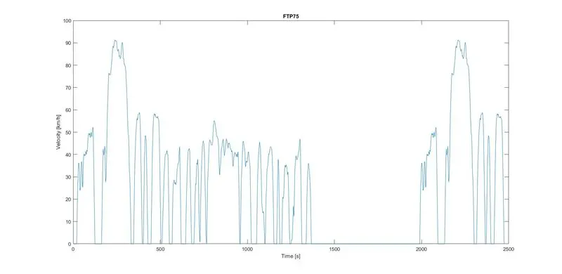
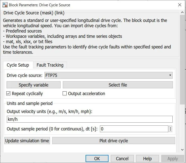
• Federal Test Procedure (FTP75):

The Federal Test Procedure (FTP) is composed of the UDDS followed by the first 505 seconds of the UDDS. Though it was originally created as a reference point for fossil fuelled vehicles, the UDDS and thus the FTP-75, are also used to estimate the range in distance travelled by an electric vehicle in a single charge.

• Wide Open Throttle (WOT) (100 Seconds):

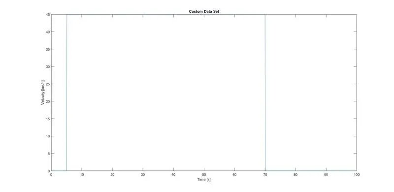
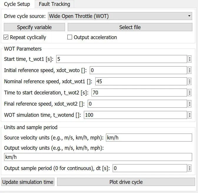
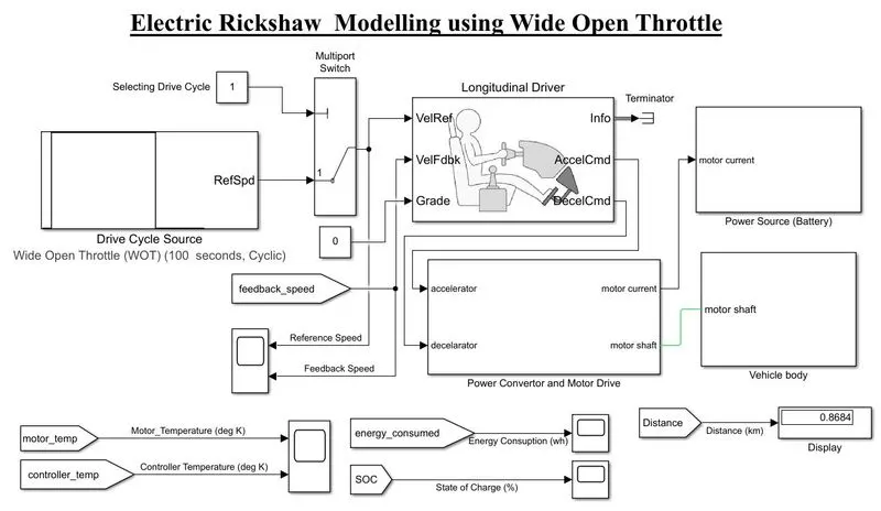
It generates a standard or user-specified longitudinal drive cycle. The block output is the vehicle longitudinal speed. Vehicle speed is 0 for first 5 second and 45kmph for 5 to 70 seconds and zero from 70 to 100 seconds.

• Signal Builder (User defined cycle):

This block is used to create and generate interchangeable groups of signals whose waveforms are piecewise linear.

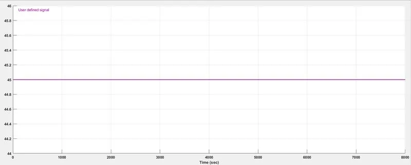
This cycle has a constant speed of 45kmph for 8000 seconds. The reason of the time being 8000 seconds is that the vehicle will take 8000 seconds for completing 100km ride at 45kmph speed.

Driver Configuration:

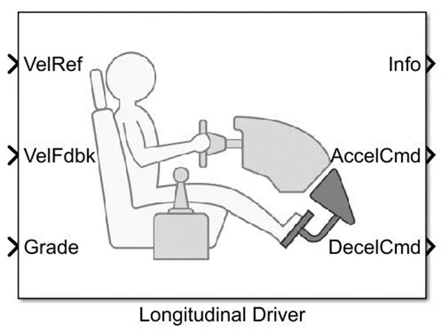
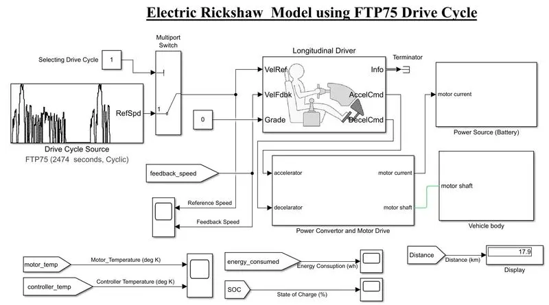
The input from the drive cycle is attached to VelRef port, the feedback is gained from the vehicle body which acts as feedback signal is connected to VelFdbk. The AccelCmd & DecelCmd are the output signal given for accelerating and braking to the vehicle. A terminator block is connected to Info port as we are not using any bus signals for this model. A constant block is attached to the Grade port as road grade angle is 0 in our case, i.e., the vehicle is running at a straight road.

• Longitudinal driver block:

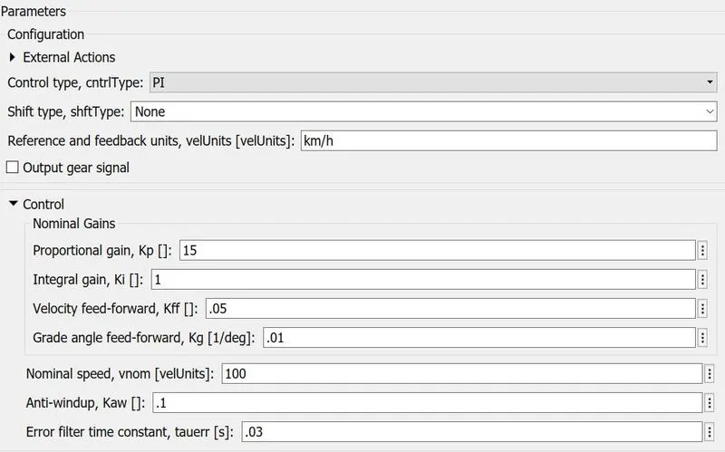
It is a parametric longitudinal speed tracking controller for generating normalized acceleration and braking commands based on reference and feedback velocities. They use the external actions to input signals that can disable, hold, or override the closed-loop commands determined by the block.

Parameters

Power Controller and Motor:

Power controller block has prime significance in the electric powertrains. It consists of controlled PWM voltage block, H-bridge block, two controlled voltage source, current sensor and temperature sensor.

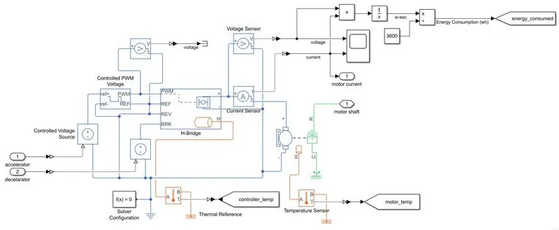
Controlled acceleration from driver subsystem is provided to controlled voltage source, the controlled voltage source converts the input of controlled acceleration signal to the equivalent voltage signal and output of controlled voltage source is provided to controlled PWM voltage block. Similarly, controlled braking signal is provided to another controlled voltage source and output of controlled voltage source is provided to H-bridge block.

• Controlled PWM Voltage:

The Controlled PWM Voltage block represents a pulse-width modulated (PWM) voltage source. The block calculates the duty cycle based on the reference voltage across its ref+ and ref- ports.

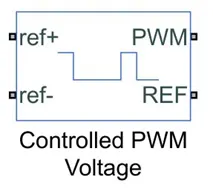
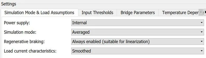
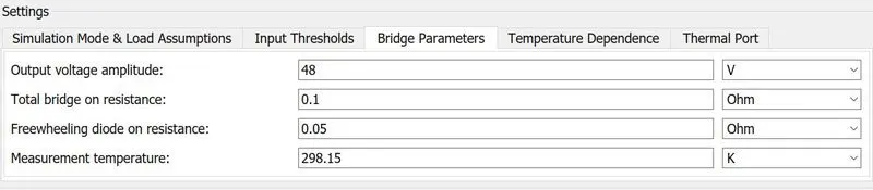
The output voltage is zero when the pulse is low, and is equal to the Output voltage amplitude parameter when high. Duty cycle is set by the input value. The Simulation mode can be set to PWM or Averaged. In PWM mode, the output is a PWM signal. In Averaged mode, the output is constant with value equal to the averaged PWM signal.

• H-bridge:

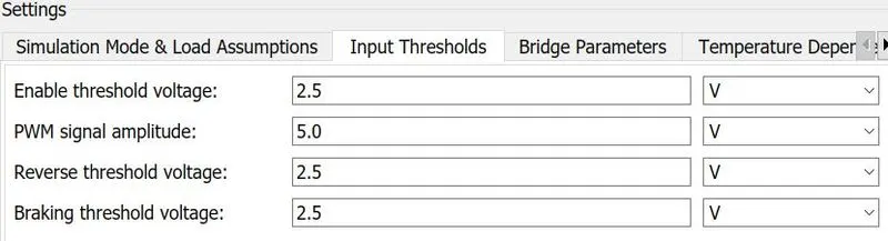
This block represents an H-bridge motor drive. The block can be driven by the Controlled PWM Voltage block in PWM or Averaged mode. In PWM mode, the motor is powered if the PWM port voltage is above the Enable threshold voltage. In Averaged mode, the PWM port voltage divided by the PWM signal amplitude parameter defines the ratio of the on-time to the PWM period.

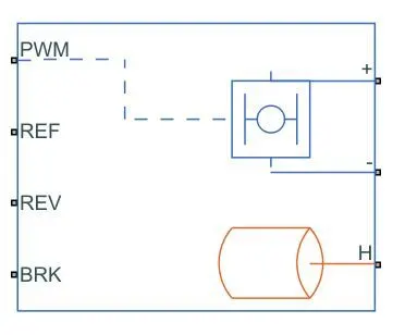
Using this ratio and assumptions about the load, the block applies an average voltage to the load that achieves the correct average load current. The signal at the REV port determines the polarity of the output. If the value of the signal at the REV port is less than the value of the Reverse Threshold Voltage parameter, the output has positive polarity; otherwise, it has negative polarity.

Simulation Mode and Load Assumptions

Input Thresholds

Bridge Parameters

Temperature Dependence

Thermal Port

• Thermal Sensor:

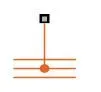
The Temperature Sensor, a device that determines the temperature differential measured between two points without drawing any heat. Connections A and B are thermal conserving ports that connect to the two points where temperature is being monitored. Port T is a physical signal port that outputs the temperature differential value. Output from H port from H-bridge block is given to port A.

The measured temperature is determined as T = TA – TB.

• DC motor:

When a positive current flows from the electrical + to - ports, a positive torque acts from the mechanical C to R ports. Motor torque direction can be changed by altering the sign of the back-emf or torque constants.

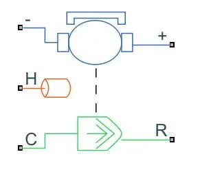
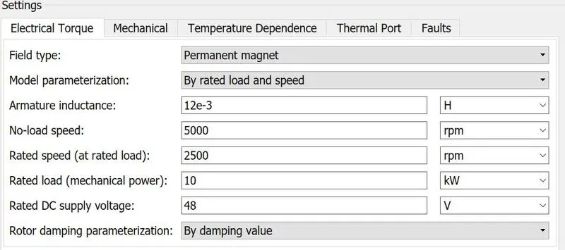
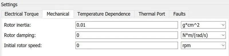
The block assumes that no electromagnetic energy is lost, and hence the back-emf and torque constants have the same numerical value Motor parameters can either be specified directly, or derived from no-load speed and stall torque. H port output from DC motor is provided to temperature sensor and shown on scope as motor Temp. Mechanical rotational reference block is used to connect mechanical rotational ports that are rigidly affixed to ground. Motor torque direction can be changed by altering the sign of the back-emf or torque constants.

Electrical Torque

Mechanical

Temperature Dependence

Thermal Port

• Energy consumption:

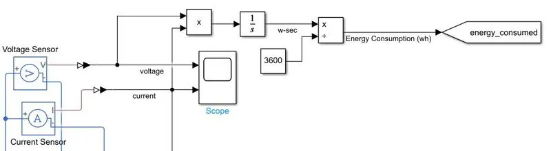
The Voltage and Current are multiplied to get the Power of the system and integrated to get the Energy (watt-sec) and converted to watt-hour by dividing with 3600.

Battery (Power Source):

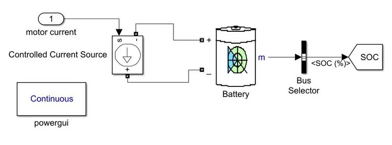
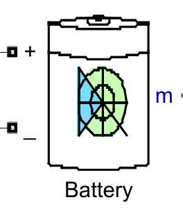
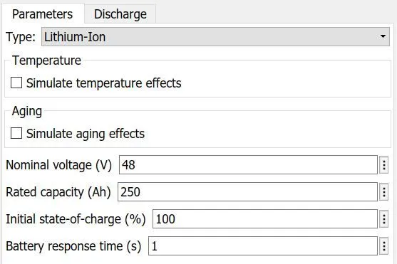
This block models a battery. If you select Infinite for the Battery charge capacity parameter, the block models the battery as a series internal resistance and a constant voltage source. If you select Finite for the Battery charge capacity parameter, the block models the battery as a series internal resistance plus a charge-dependent voltage source defined by:

V=Vnom * SOC1−β⋅(1−SOC)

where, SOC is the state of charge

Vnom is the nominal voltage.

Coefficient β is calculated to satisfy a user-defined data points.

• Controlled Current Source

Converts the Simulink input signal into an equivalent current source. The generated current is driven by the input signal of the block.

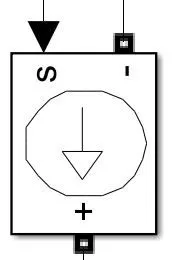
You can initialize your circuit with a specific AC or DC current. If you want to start the simulation in steady-state, the block input must be connected to a signal starting as a sinusoidal or DC waveform corresponding to the initial values

Vehicle Dynamics:

Vehicle dynamics subsystem is simply the vehicle body working to the given task. It has wheels road conditions, surrounding conditions, load on the vehicle etc.

This subsystem represents the 3-wheeler vehicle body with the transmission.

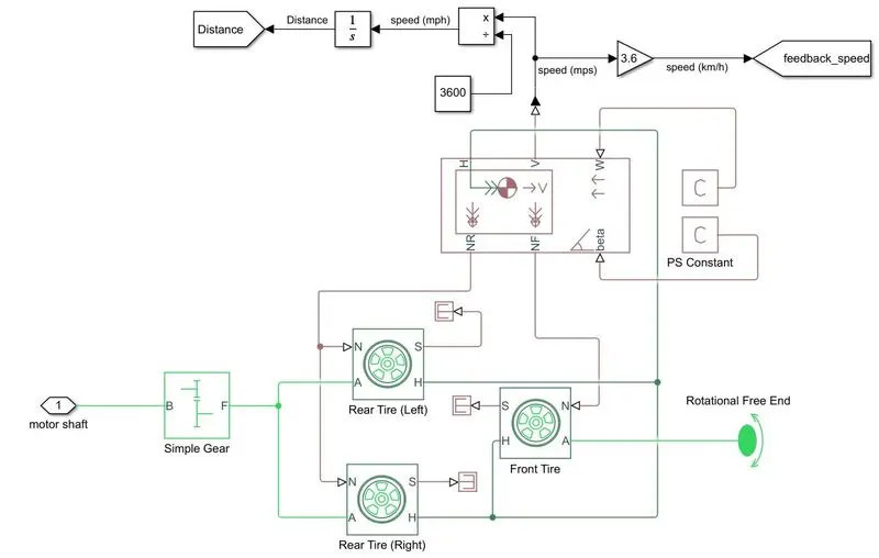
A set of three tire block are used - one for the front free rotation and two for the rear axle and the required connections are made with the vehicle body block. The normal force signal from the vehicle body block is sent to the normal force input ports of the tires.

The A ports of the tire are the mechanical rotational conserving port and receive mechanical rotational input from the gearbox which receives its input from the DC motor.

The H port of the tire is the mechanical translational conserving port for the wheel hub and is connected to the H port of the vehicle body through which the trust developed by the tire is applied to the vehicle.

Here we are not considering any slip, so a terminator block is connected to all the slip port of each tire. Also, grade angle and wind velocity are not considered.

The input is received from the DC motor to the simple gear block which is then transmitted to the wheel considering the inertia couple at the output shaft.

• Gear Box:

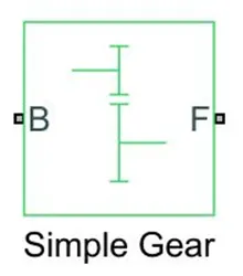
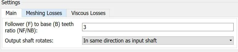
The gear box is characterized by its Gear ratio. The gear ratio is determined as the ratio of the input shaft angular velocity to that of the output shaft. Here Gear ratio is 3.

The gear ratio set as 3. The more the gear ratio the better the speed with more traction power. As torque is directly proportional to the speed. The gear ratio is high at the start of the vehicle as it requires more torque and as the speed increases, torques reduces and so as the gear ratio.

• Vehicle body:

Represents a two-axle vehicle body in longitudinal motion. The block accounts for body mass, aerodynamic drag, road incline, and weight distribution between axles due to acceleration and road profile. Optionally include pitch and suspension dynamics or additional variable mass and inertia. The vehicle does not move vertically relative to the ground.

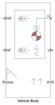
Connection H is the mechanical translational conserving port associated with the horizontal motion of the vehicle body. The resulting traction motion developed by tires should be connected to this port. Connections V, NF, and NR are physical signal output ports for vehicle velocity and front and rear normal wheel forces, respectively. Wheel forces are considered positive if acting downwards. Connections W and beta are physical signal input ports corresponding to headwind speed and road inclination angle, respectively. If variable mass is modelled, the physical signal input ports CG and M are exposed. CG accepts a two- element vector representing the x and y distance offsets from vehicle CG to additional load mass CG. M represents the additional mass. If both variable mass and pitch dynamics are included, the physical signal port J accepts the inertia of the additional mass about its own CG.

Main

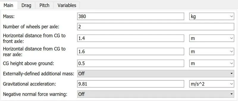
The weight of the vehicle is considered as 380 kg and rest of the parameters are same as default.

Drag

The vehicle Frontal area is set as 2.36 square meters and Drag Coefficient as 0.3 and air density of 1.18 km/m^3.

• Tire (Magic formula):

The block represents the longitudinal behaviour of a highway tire characterized by the tire Magic Formula. The block is built from Tire-Road Interaction (Magic Formula) and Simscape Foundation Library Wheel and Axle blocks. Optionally, the effects of tire inertia, stiffness, and damping can be included.

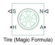
Tyre block Represents the longitudinal behaviour of a highway tire characterized by the tire Magic Formula. Connection A is the mechanical rotational conserving port for the wheel axle. Connection H is the mechanical translational conserving port for the wheel hub through which the thrust developed by the tire is applied to the vehicle. Connection N is a physical signal input port that applies the normal force acting on the tire. The force is considered positive if it acts downwards. Connection S is a physical signal output port that reports the tire slip. Optionally expose physical signal port M by right-clicking on the block and selecting Simscape block choices to switch between variants. Physical signal port M accepts a four-element vector corresponding to the B, C, D, and E Magic Formula coefficients.

Main

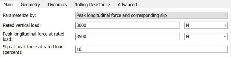
The tire is parameterized by peak longitudinal force and corresponding slip and rest of the parameters are keep as same as default.

Geometry

Rolling radius of the tire is 0.16 m

Rolling Resistance

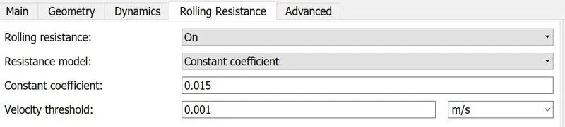
Rolling resistance is ‘on’ with constant coefficient of 0.015.

• Rotational Free End:

This block represents a mechanical rotational free end. Use it to allow a node to rotate freely without torque. This block can be used to optionally specify initial rotational velocity.

• Distance Calculation:

The output of the vehicle body is Velocity, which is sent as feedback_speed to the longitudinal driver block and is separately used to calculate the distance travelled by the Vehicle.

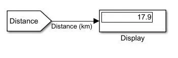
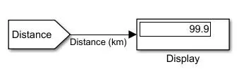
The velocity signal (m/s) is first integrated to calculate the distance and then divide by 1000 to convert the distance into km.

RESULTS:

Case-1: Electric Rickshaw Model using FTP75 Dive Cycle:

Comparing Reference Speed and Feedback Speed:

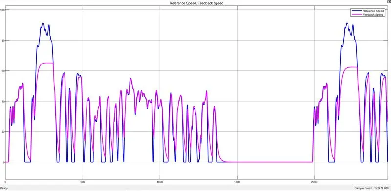
The modelled rickshaw almost follows the given input drive cycle.

Comparing Motor and Controller temperatures:

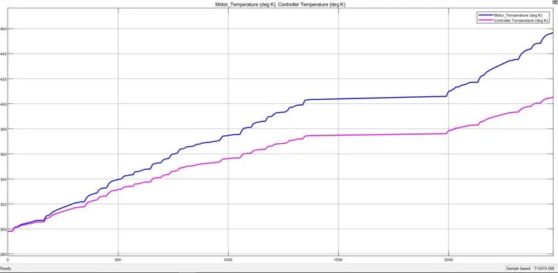
Motor temperature increased for 298 deg. K to 455 deg. K when in operation. This rise of temperature is very high and need to be controlled. It can be concluded by cooling mediums and cooling is necessary for this powertrain for efficient working and durability.

Temperature of controller rises when the vehicle is running and is constant when it stops. Rise in Temperature is less compared to Motor.

SOC:

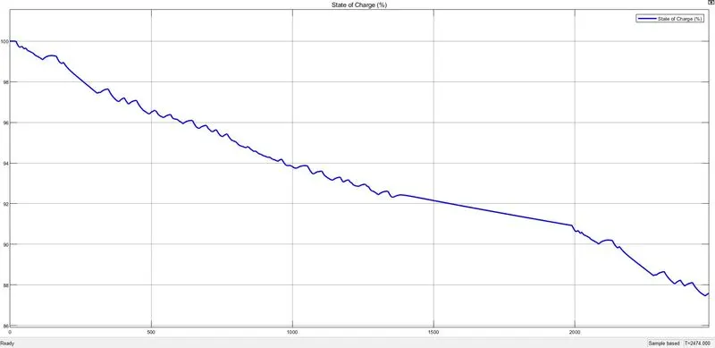
SOC was 100% at start of the drive and is reduced to 87.5%, SoC plot is constant whenever vehicle is stopped and rise in the curve is seen due to regenerative braking.

Comparing Voltage and Current:

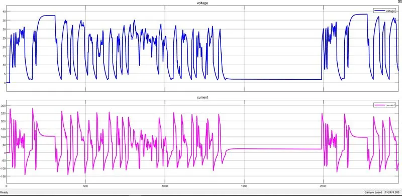
AS per the drive current follows positive and negative profile. Positive being current drawn from the battery and negative being current drawn inside the battery (regeneration). That is where the SOC increases. Also, it is zero for zero speed between 1400 and 2000 seconds (approx.) span.

Energy Consumption:

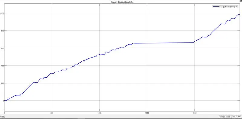
Overall energy consumed is 985 wh

Distance travelled by the Vehicle:

Case-2: Electric Rickshaw Model using WOT (Wide Open Throttle):

Comparing Reference Speed and Feedback Speed:

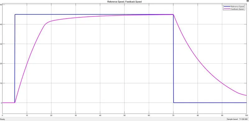
The feedback speed tried to follow the reference speed and before reaching the specified speed throttle was released from full to zero. The rickshaw could not reach reference speed of 45kmph within 70 seconds. Also, to reach zero after wot is released, it took next almost 35 seconds to reach zero (to stop).

Comparing Motor and Controller temperatures:

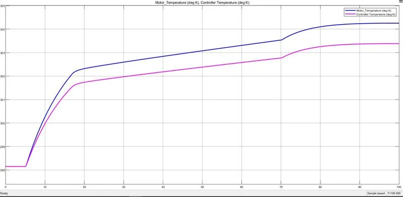
The Motor temperature increased from 298.2 deg. K to 304.4 deg. K.

Temperature of controller is constant for first 5 seconds as there is no input and vehicle is at rest. As the vehicle starts to follow the WOT condition, the temperature drastically increases. When it reaches above 45kmph and now tries to settle, temperature is also settled to some extent and no rise is seen in it. Again, during deceleration same behaviour is seen. Rise in Temperature is negligible.

SOC:

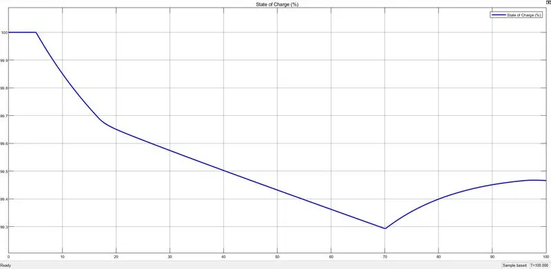
At constant speed (Zero), SOC is 100% for first 5 seconds. As vehicle starts running for 70 seconds, SOC drops to 99.29% and then again rises back to 99.47 in next 30 second as brakes are applied.

Comparing Voltage and Current:

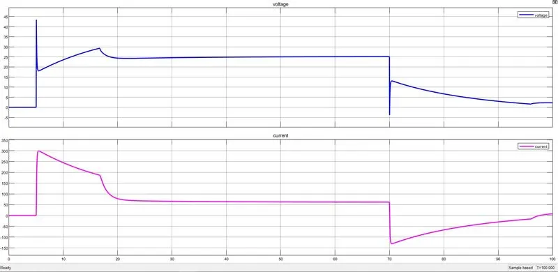
For current, it is zero for zero speed (at rest), positive (drawn from battery) till 70 seconds and it is negative (drawn to battery) for 70 to 100 seconds.

Energy Consumption:

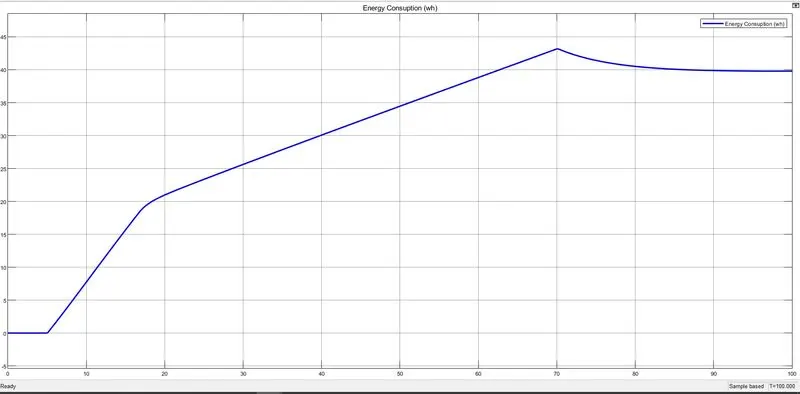
At the start of 5 seconds no energy is required. From 5 seconds to the 70 seconds the requires energy is 43 wh and after 70 seconds the vehicle will decelerate to the required energy will decrease gradually.

Distance travelled by the Vehicle:

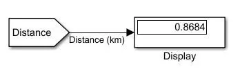
Case-3: Electric Rickshaw Model using Signal Builder (User Defined Signal):

Comparing Reference Speed and Feedback Speed:

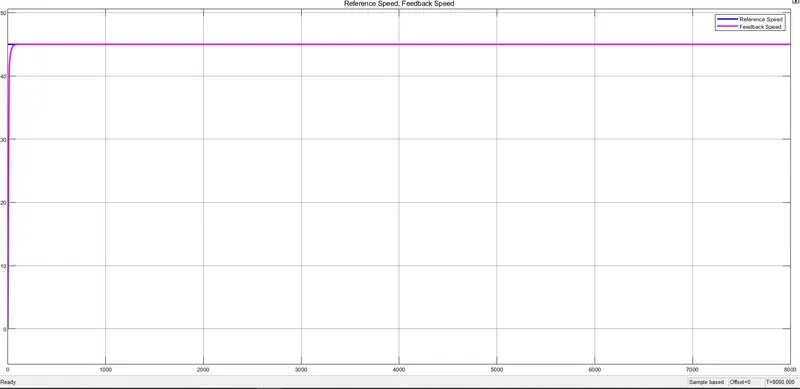
Above plot describes the control accuracy of the system up to 8000 seconds. Input speed and output speed is very identical, meaning the controller is performing its function accurately. Constant speed of 45 kmph is achieved throughout the 100km distance

Comparing Motor and Controller temperatures:

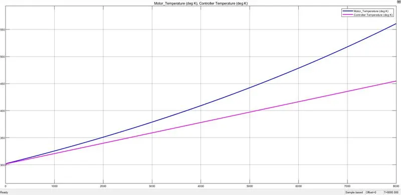
For 0 to 45kmph acceleration, Motor temperature rise was from 298 to 560 deg. k

During the 100km travel of the vehicle at constant 45 kmph speed, the controller temperature has risen from 298.15 to 455 deg. k.

SOC:

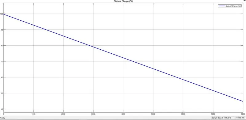
The SOC for the Vehicle was 100% at beginning, reached to 45% at the end of 100km. We can notice that the there was no rise in SOC because no regeneration action taking place.

Comparing Voltage and Current:

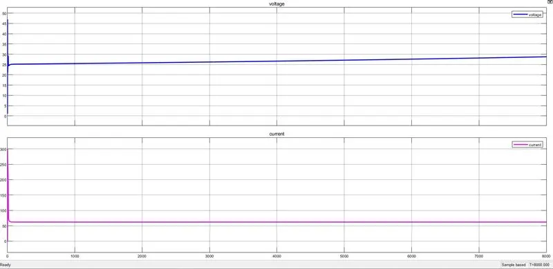
The current drawn from the battery is also constant throughout. Also, the current is only in positive direction. This is because the speed never changes and there is no deceleration. If there was any deceleration, there would be current regeneration and battery would be charged resulting in negative current.

Energy Consumption:

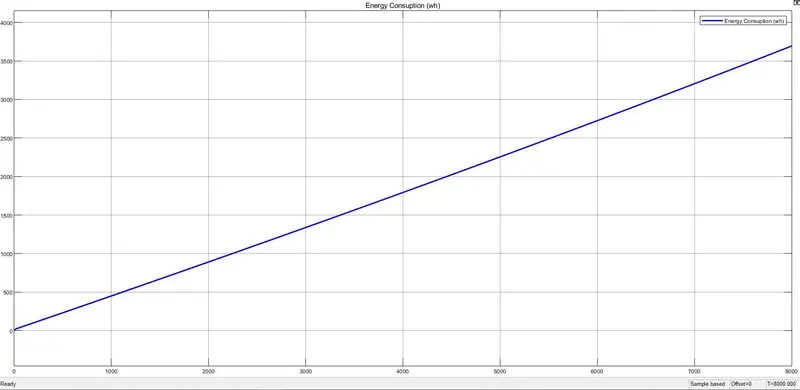3700 wh of Energy have been consumed

Distance travelled by the Vehicle:

Comparing the three cases:

Parameters / Cases	Case-1: FTP75	Case-1: FTP75	Case-1: FTP75
% Match in reference and feedback speed	75	65	97
Motor Temperature (Kelvin)	457	304.3	560
Controller Temperature (Kelvin)	407	303.4	452
SOC (%) at the end of the drive cycle	87.5	99.47	45
Energy Consumed (Wh)	990	39	3700
Distance Travelled (Km)	17.9	0.8684	99.9

CONCLUSION:

We have modelled the Electric Rickshaw and studied for thee drive cycles and absorbed variation in temperature of Motor and Controller, SOC and Energy Consumed by the vehicle for all the three Drive cycles.

If we consider the real time application, the motor, battery & controller temperature is controlled by different cooling technologies. So, there temperatures can be controlled. Here we need compromise with the temperature of Motor and Controller to achieve vehicle speed is near to reference speeds.

Finally, observed the temerature rise in motor and controller when the vehicle runs for 100 Km with constant speed of 45kmph for drive time of 8000 seconds.

REFERENCES:

https://www.gemev.com/electric-rickshaw.html

Drive Link:

https://drive.google.com/drive/folders/1Bc9VB34KvCZ82NFmXS7t7lcePxltC2lV?usp=sharing