Final Project: Design of an Electric Vehicle
Electric Vehicle Design of IHEV
AIM : To Create a MATLAB model of electric car which uses a battery and a DC motor. Choose suitable blocks from Powertrain block set and to Prepare a report about the model.
solution:
objectives of the model:
1)To design a most simple electric vehicle model using individual component models.
2)To check the performance parameters of vehicle like speed. battery soc, distance.
3)To know how the different parameters are configured based on the vehicle requirement.
4)To know the MATLAB models and their configuration to match with actual vehicle.
System level configurations
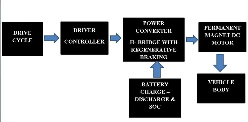
At system level the required components are
1)Permanent Magnet Dc motor
2)Battery source
3)H - Bridge Power Converter
4)Driver Controller
5)Vehicle body
6)Drive cycle
Block Diagram For The Model:
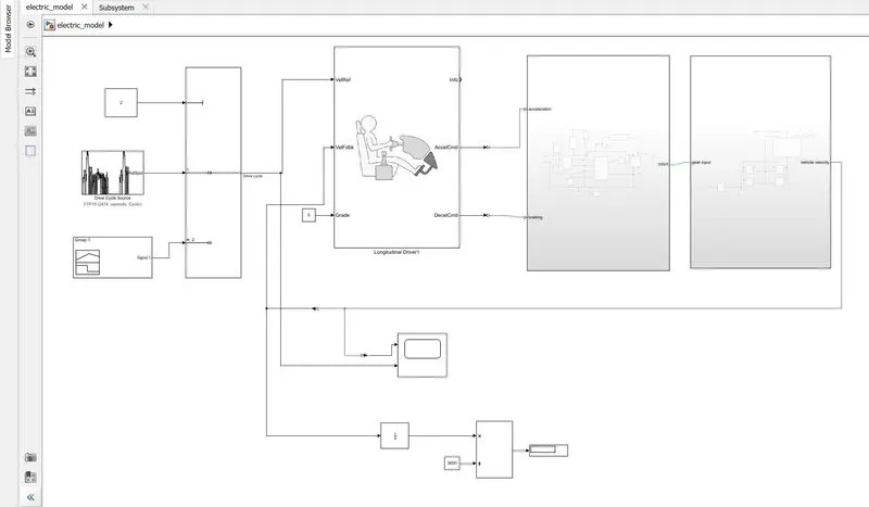
MATLAB model of Electric car which uses a battery and a DC motor:
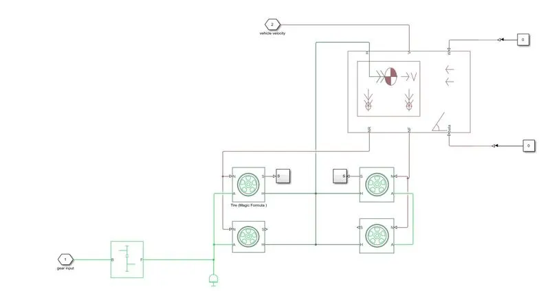
Vehicle Subsystem (or)Mechanical/Drive Train Plant:
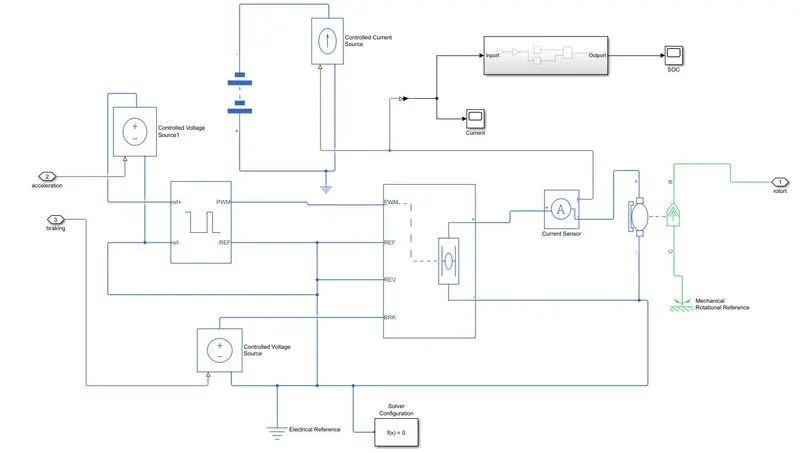
Electical SubSystem:
Battery SOC Subsystem:
Description and Procedure Of Designing The Model:
Step 1: Considering a vehicle body with chasis where the inputs or connecting ports of the vehicle are connected with the tyres . we can configure the vehicle body with parameters like weight, frontal area,no of wheels,drag coefficient etc. where the body is coming with Inputs like the wind velocity, inclination angle and vehicle velocity which are assigned with the values accordingly and other inputs like NR,NF(normal force) connected to the rear axle and front axles.
Step 2: The front and rear axles of the tyres are connected together and also to vehicle body the configuration of the tyres according to the magic formula is choosen like slip,rolling radius,rolling resistance and dynamics etc.once we have the 4 wheels connected to the vehicle body .
Part of gear system a simple gear is connected to the rear axle where the ouput of gear system is connected to rear axle and the input is connected to the shaft of the motor. so the vehicle body with tyres and gear system are made as a sub system and we can name as mechanical or drivetrain part of the model.
Step 3:Now coming to the electric part of the model we have chossen a brush type dcmotor where the input of the motor is connected with the power converter output and the output of the motor is already connected with the gear system and also a rotational reference frame is connected with the casing port of motor.
The parameters which can be choosed in dc motor like rated power, rated speed,no load speed,armature inductance,rated dc supply usually these motors are high power and high voltage in this way the motor is configured with the given parameters. The dc motor will acts as a generator for shorter duration of time in regenerative breaking mode and feeds the battery with negative currrent whenever the vehicle is slowing down.
Step 4:For controlling the motor we have taken a H Bridge converter which is a combination of 4 no of switches so, now we have a PWM controlled dc motor drive. H Bridge can be configured in multiple no of ways by changing the parameters like simulation mode, input thresold values and bridge parameters like ouput voltage amplitude. Here the H Bridge output is connected with the motor.
Step 5: Now we have to know how we are controlling the H BRIDGE for that we have to connect the H Bridge input to controlled PWM voltage source output this source is actually going to apply pulses and based on the pulses from fixed battery voltage the variable battery voltage is available as an input to the motor so, based on the variable voltage the motor speed and torque is controlled. Now the H Bridge is going to receive control signals from the controller.
Step 6: We require a controlled voltage source blocks for connecting the controlled PWM voltage sorce as input and also to the braeak input of H bridge for regenerative breaking so when ever the vehicle speed is reduced the power can go back to the battery and the battery will get charged.
Step 7: For giving the control signals we need a speed data prior to running the simulation which changes w.r.t time can be obtained by a driving cycle souce and this is actually a speed vs time data where we can choose no of drive cycles and also we can create our own drive cycle with excel data sheet .This drive cycle source gives some standard drive cycles followed by automobile manufacaturing companies based on these drive cycles the vehicle mileage and performance is tested.
Step 8: we are taking this drive cycles as pre defined vehicle input. Now this drive cycles data is to be converted into the acceleration and deceleration commands which are to be applied to controlled voltage source block as acceleration input and deceleration command to brake input of H Bridge converter. In place of drive cycle source we can have a signal buider block to have our own drive cycle which is also used in this model.
Step 9: we have a longitudinal driver who is going to convert the drive cycle input into acceleration and deceleration commands for that based on the velocity reference that he gets from the drive cycle source and the driver here is constantly following the vehicel reference speed and it will be compared with the vehicel feedback speed obtained from the vehicel model. where the velocity input of the vehicel body is connected to the vehicle feedback of driver.
Here the driver compares the two speeds of drive cycle and the vehicle feedback. so if the targeted speed is more than the vehicle actual speed then the driver press the accelerator then the acceleration commands reach the controller to converter and the voltage is increased accordingly the pulse signals which increases the motor speed and torque or If the targeted speed is less than the vehicle actual speed then the driver press the brake pedal then the deceleration commands reach the converter and the voltage is deccreased accordingly the pulse signals which deccreases the motor speed and torque.
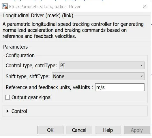
Step 10: Here the longitudinal driver works on PI controller type and from the control parameters in this block we can configure this driver block which results in the generation of accelearation and deceleration or brake commands. This driver is a logic part where the signals will be coming out like 0 and 1 which is given to controller.
Step 11: we are going to connect the battery in such away that it is going to get discharge according to the currrent taken out from the dc motor. we are connected the battery to controlled current source which will discharge the battery according to the current taken out from the motor.
Step 12: We have connected a current sensor with battery, converter and the motor so we can charge and discharge the battery according to the current taken out and coming in from the motor when it acts as a generator.
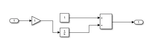
Step 13: we have connected a solver configuration block, electrical referene to the system and we used a integrator block to convert the speed into distance and for knowing the battery state of charge (soc) we have made a sub system. With this the model arrangement and connection procedure is completed.
The Model parameters used in this model are:
1)Drive cycle source:
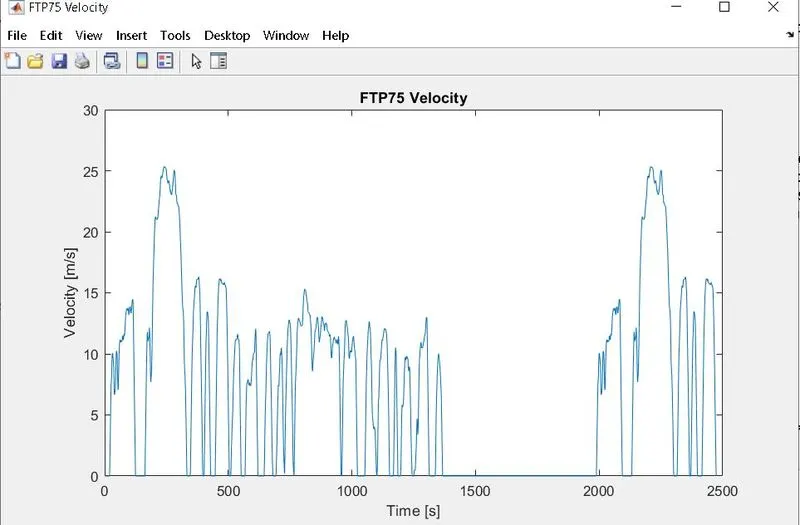
This block generates standard or user specified drive cycles i.e velocity vs time. There are many types of different drive cycles by considering different drive cycles we can test the vehicle performance and the power required. In this case I have used a FTP 75 standard drive cycle for 2474 seconds.FTP75 drive cycle is kept as the vehicle input drive cycle from the default drive cycle keeping all the other parameters same and the output result as vehicle behaviour is known by this drive cycle.From this block we can choose or input various drive cycles or the parameters can be changed
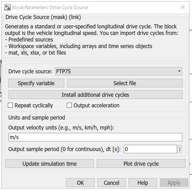
This was the FTP75 drive cycle the vehicle performance is tested based on this drive cycle.
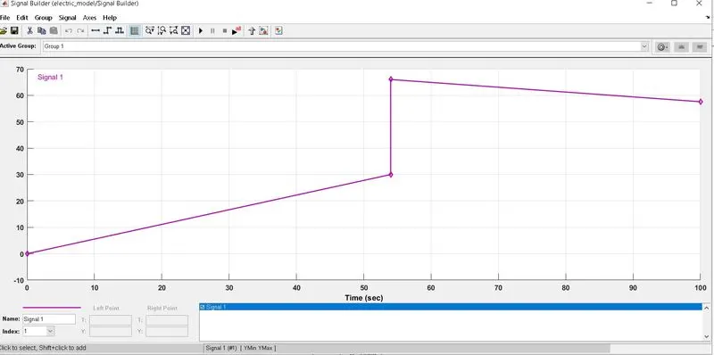
Drive cycle 2 as Signal Builder Block:
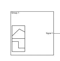
This is how we build our own signals where y axis and x axis can be changed to our requirement
2)Longitudinal driver:
It is a simulated driving environment which follows the velocity input or This works based on the velocity reference(Vref) and velocity feedback (Vfb) as inputs, it’s a speed tracking controller and generates acceleration and braking commands as output to the controller. Longitudinal driver acts in such away that the difference between the velocity reference and velocity actual is minimised.From this block the variables can be changed like changing control type
3)Scope:
Scope displays the output of the model with the corresponding inputs given to the model, scope varies with the change in the model parameters.
4)Dc motor:
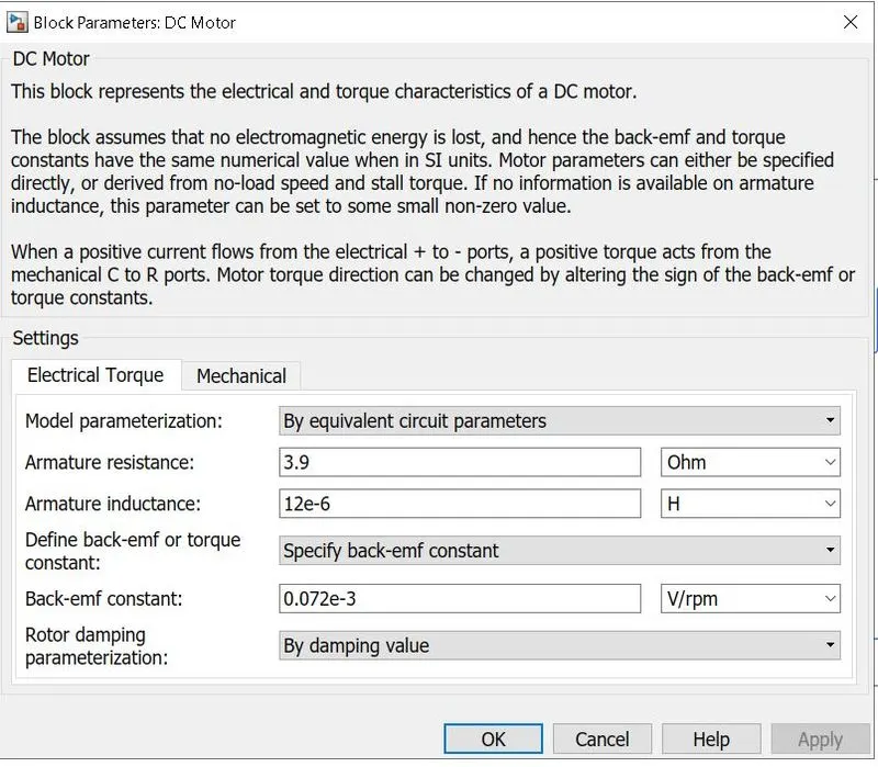
This block represents the electrical and torque characteristics of a DC motor.
The block assumes that no electromagnetic energy is lost, and hence the back-emf and torque constants have the same numerical value when in SI units. Motor parameters can either be specified directly, or derived from no-load speed and stall torque. If no information is available on armature inductance, this parameter can be set to some small non-zero value.
When a positive current flows from the electrical + to - ports, a positive torque acts from the mechanical C to R ports. Motor torque direction can be changed by altering the sign of the back-emf or torque constants. From this block the variables can be changed like changing the variables like motor resistance, inductance and others.
5)Controlled voltage source:
The Controlled Voltage Source block converts a Simulink input signal into an equivalent voltage source. The generated voltage is driven by the input signal of the block. You can initialize the Controlled Voltage Source block with a specific AC or DC voltage.
The block represents an ideal voltage source that is powerful enough to maintain the specified voltage at its output regardless of the current passing through it. The output voltage is V = Vs, where Vs is the numerical value presented at the physical signal port.
6)Controlled current source:
The Controlled Current Source block converts the Simulink input signal into an equivalent current source. The generated current is driven by the input signal of the block. The positive current direction is as shown by the arrow in the block icon.The block represents an ideal current source that is powerful enough to maintain the specified current through it regardless of the voltage across it. The output current is I = Is, where Is is the numerical value presented at the physical signal port.
7)H Bridge converter:
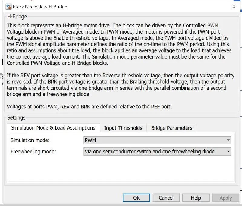
This block represents an H-bridge motor drive. The block can be driven by the Controlled PWM Voltage block in PWM or Averaged mode. In PWM mode, the motor is powered if the PWM port voltage is above the Enable threshold voltage. In Averaged mode, the PWM port voltage divided by the PWM signal amplitude parameter defines the ratio of the on-time to the PWM period. Using this ratio and assumptions about the load, the block applies an average voltage to the load that achieves the correct average load current. The Simulation mode parameter value must be the same for the Controlled PWM Voltage and H-Bridge blocks.
If the REV port voltage is greater than the Reverse threshold voltage, then the output voltage polarity is reversed. If the BRK port voltage is greater than the Braking threshold voltage, then the output terminals are short circuited via one bridge arm in series with the parallel combination of a second bridge arm and a freewheeling diode.Voltages at ports PWM, REV and BRK are defined relative to the REF port.
From this block we can change the variables ike no of semiconductor switches and free wheeling dioded,threshold values, bridge parameters like output voltage amplitude
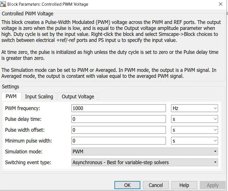
8)Controlled PWM voltage:
This block creates a Pulse-Width Modulated (PWM) voltage across the PWM and REF ports. The output voltage is zero when the pulse is low, and is equal to the Output voltage amplitude parameter when high. Duty cycle is set by the input value. Right-click the block and select Simscape->Block choices to switch between electrical +ref/-ref ports and PS input u to specify the input value.
At time zero, the pulse is initialized as high unless the duty cycle is set to zero or the Pulse delay time is greater than zero.
The Simulation mode can be set to PWM or Averaged. In PWM mode, the output is a PWM signal. In Averaged mode, the output is constant with value equal to the averaged PWM signal.
The Controlled PWM Voltage block represents a pulse-width modulated (PWM) voltage source.
From this block the variables can be changed like PWM frequency,delay time ,pulse width,duty cycle and output voltage amplitude.
9)Current sensor:
The Current Sensor block represents an ideal current sensor, that is, a device that converts current measured in any electrical branch into a physical signal proportional to the current. Connections + and – are electrical conserving ports through which the sensor is inserted into the circuit.
10)Mechanical rotational reference:
The Mechanical Rotational Reference block represents a reference point, or frame, for all mechanical rotational ports. All rotational ports that are rigidly clamped to the frame (ground) must be connected to a Mechanical Rotational Reference block.
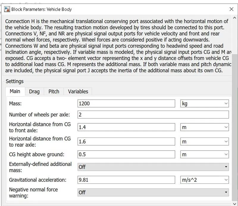
11)Vehicle body:
Represents a two-axle vehicle body in longitudinal motion. The block accounts for body mass, aerodynamic drag, road incline, and weight distribution between axles due to acceleration and road profile. The vehicle can have the same or a different number of wheels on each axle. Optionally include pitch and suspension dynamics or additional variable mass and inertia. The vehicle does not move vertically relative to the ground.
Connection H is the mechanical translational conserving port associated with the horizontal motion of the vehicle body. The resulting traction motion developed by tires should be connected to this port. Connections V, NF, and NR are physical signal output ports for vehicle velocity and front and rear normal wheel forces, respectively. Wheel forces are considered positive if acting downwards. Connections W and beta are physical signal input ports corresponding to headwind speed and road inclination angle, respectively. If variable mass is modeled, the physical signal input ports CG and M are exposed. CG accepts a two- element vector representing the x and y distance offsets from vehicle CG to additional load mass CG. M represents the additional mass. If both variable mass and pitch dynamics are included, the physical signal port J accepts the inertia of the additional mass about its own CG.
From this block all the vehicle related variables are selected and changed to the requirement.
12)Tires:
Represents the longitudinal behavior of a highway tire characterized by the tire Magic Formula. The block is built from Tire-Road Interaction (Magic Formula) and Simscape Foundation Library Wheel and Axle blocks. Optionally, the effects of tire inertia, stiffness, and damping can be included.
Connection A is the mechanical rotational conserving port for the wheel axle. Connection H is the mechanical translational conserving port for the wheel hub through which the thrust developed by the tire is applied to the vehicle. Connection N is a physical signal input port that applies the normal force acting on the tire. The force is considered positive if it acts downwards. Connection S is a physical signal output port that reports the tire slip. Optionally expose physical signal port M by setting Parameterize by to Physical signal Magic Formula coefficients. Physical signal port M accepts a four element vector corresponding to the B, C, D, and E Magic Formula coefficients.
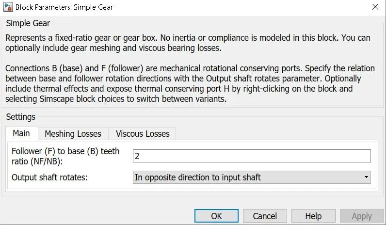
13)Simple gear:
Represents a fixed-ratio gear or gear box. No inertia or compliance is modeled in this block. You can optionally include gear meshing and viscous bearing losses.
Connections B (base) and F (follower) are mechanical rotational conserving ports. Specify the relation between base and follower rotation directions with the Output shaft rotates parameter. Optionally include thermal effects and expose thermal conserving port H by right-clicking on the block and selecting Simscape block choices to switch between variants.From this block the gear related variables are changed.
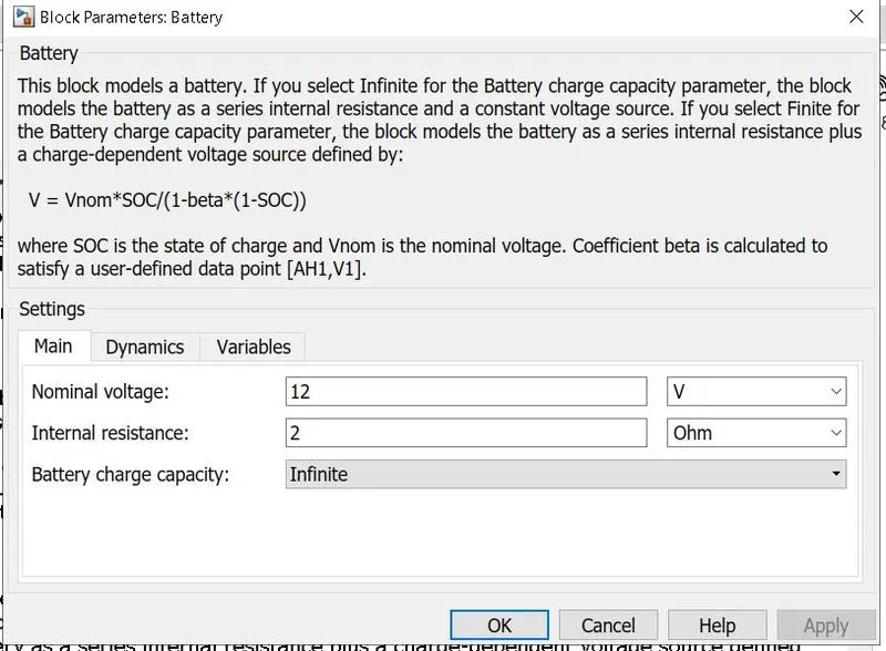
14)Battery source:
This block models a battery. If you select Infinite for the Battery charge capacity parameter, the block models the battery as a series internal resistance and a constant voltage source. If you select Finite for the Battery charge capacity parameter, the block models the battery as a series internal resistance plus a charge-dependent voltage source defined by: V = Vnom*SOC/(1-beta*(1-SOC))
where SOC is the state of charge and Vnom is the nominal voltage. Coefficient beta is calculated to satisfy a user-defined data point [AH1,V1]. From this block the battery variables are changed.
15)Inertia block:
By default, the block has one mechanical translational conserving port. The block positive direction is from its port to the reference point. This means that the inertia torque is positive if inertia is accelerated in positive direction.
16)Electrical Reference:
The Electrical Reference block represents an electrical ground. Electrical conserving ports of all the blocks that are directly connected to ground must be connected to an Electrical Reference block. A model with electrical elements must contain at least one Electrical Reference block.
17)Mechanical Rotational Reference:
The Mechanical Rotational Reference block represents a reference point, or frame, for all mechanical rotational ports. All rotational ports that are rigidly clamped to the frame (ground) must be connected to a Mechanical Rotational Reference block.
18)Solver Configuration:
Each topologically distinct Simscape block diagram requires exactly one Solver Configuration block to be connected to it. The Solver Configuration block specifies the global environment information and provides parameters for the solver that your model needs before you can begin simulation.
RESULTS:
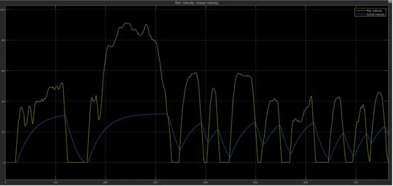
SIMULATION OUTPUT RESULT OF DRIVE CYCLE INPUT:
From the result we can observe the vehicle actual velocity is trying to follow the vehicle drive cycle input or reference velocity but it is lesser bcause of the model parameters which are given to the model and this can varied by giving the requied inputs as parameters so the actual velocity can match the reference velocity.
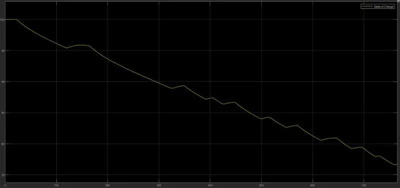
SIMULATION OUTPUT RESULT OF BATTERY SOC:
From the output result we can observe the decrease in the battery state of charge along with the distance covered by the vehicle.
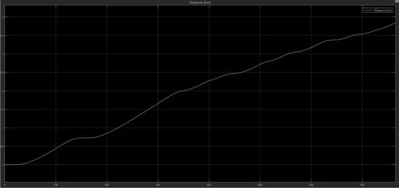
SIMULATION OUTPUT RESULT OF DISTANCE TRAVELLED :
From the output result we can observe the distance covered by the vehicle from initial zero speed till the end of the drive cycle .
CONCLUSION:
1)Based on the results we acheived our objectives of developing the most simple electric vehicle model using individual components models or blocks taken from simulink,simscape,power train block set library of matlab.
2)The performance parameters are checked like vehicle speed, battery soc, distance .
3)By configuring different parameters which are related to motor,converter,controller,vehicle body,drive cycle,battery we are able to design a electricvehicle model according to the deisign requirements.
4)Finally the designed vehicle is tested and simulated by using MATLAB to match with actual vehicle with the ouput result we can analyze and come to a conclusion that the vehicle model requires more power to actually match the drive cycle input.