Final Project: Design of an Electric Vehicle

                                                               Design of an Electric Vehicle

Abstract:

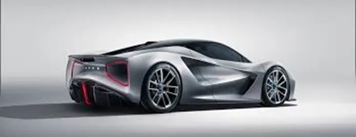
Electric vehicles are by many seen as the cars of the future as they are very efficient, produce no local pollution, are silent, and can be used for power regulation by the grid operator. In order to be able to estimate the performances of an electric vehicle it is very important to have a proper model of it. The electric vehicle model is very complex as it contains many different components. Each component needs to be modelled properly in order to prevent wrong conclusions. The design or rating of each component is a difficult task as the parameters of one component affect the power level of another one. There is therefore a risk that one component is rated inappropriately which may make the vehicle unnecessary expensive or inefficient. In this project a new design model of the electric vehicle is presented. This model is based on the Powertrain blockset using MATLAB simulation. MATLAB simulation has been used to model and simulate the electric vehicle and has been used to optimize the design variables. The model ensures that the requirements related to driving distance and acceleration are fulfilled.

Introduction:

With the considerable development of the mechanic industry, means of transportation are increasingly numerous. The car remains the most coveted locomotion. There are two major types of vehicles: the usual cars which are equipped with a combustion engine and those which are electric. The electric car has not yet replaced the gasoline car. This type of vehicle has various disadvantages, particularly in terms of cost, autonomy, supply and speed. Indeed, the production of different parts of the car is much more complicated, the cost becomes necessarily higher and the battery is drained within few hours. The battery recharging should be carried out approximately every 100 km. These drawbacks are not so far definitive. The increase in fuel prices and emission standards require new technologies that are developed to meet these needs. At the same time, the automotive industry needs always to satisfy its customers by keeping up a high-performance standard. For that, manufacturers are trying to find away to fix it, having the hope that the electric car can win in the near future the heart of consumers. Preliminary design of electric vehicle can be performed using different tools such as multi-domain, MATLAB/Simulink etc., Several studies were performed to improve and optimize models of electric vehicles in order to obtain a more reliable and more efficient vehicle.

In this project, we propose a new model for the preliminary design of an electric vehicle. The proposed mode is based on the MATLAB Simulation using Powertrain Blockset library. MATLAB Simulation has been used to model and verify the proposed model. The optimization of design variables has been performed using algorithms available in Powertrain blockset and Simulink libraries.

 

Modelling of Electric vehicle:

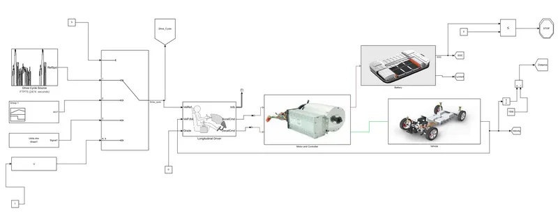
Different models of an electric vehicle exist as there are many possibilities depending on the type of the electric machine (DC or AC motor), the nature of the inverter (single or three phase) and the characteristics of the battery (high or low voltage). In this project, the electric vehicle model has been modelled using MATLAB Simulation. This model is composed of the following components a battery (DC voltage source), a rectifier (DC-DC inverter), an electric machine (DC motor), a Vehicle body, a resistive force and a control system. A current sensor, a voltage sensor, and a SoC component are used to measure respectively the electric current generated by the battery, the vehicle velocity and the State-of-Charge of the battery.

Blocks Used for Modelling:

Signal Builder:

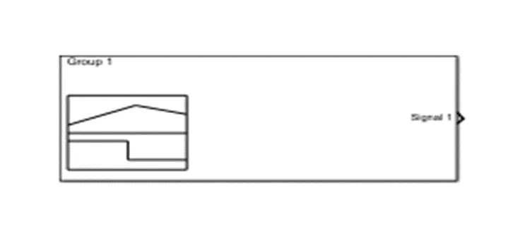
The Signal Builder block allows you to create interchangeable groups of piecewise linear signal sources and use them in a model. You can quickly switch the signal groups into and out of a model to facilitate testing. In the Signal Builder window, create signals and define the output waveforms.

 

 

Drive cycle source:

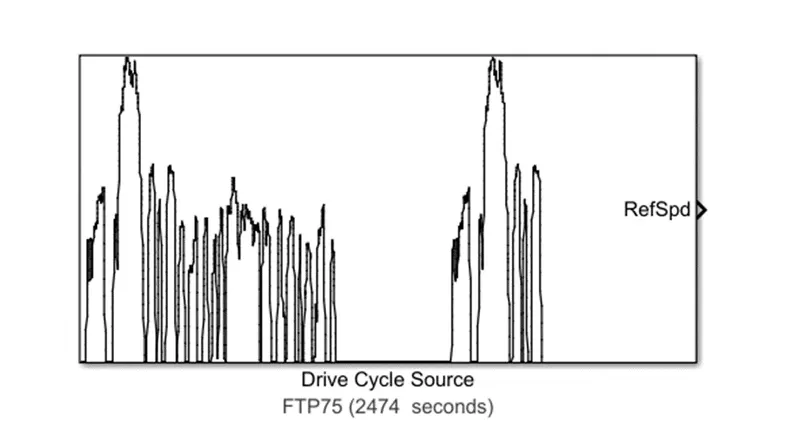
Driving cycle is a velocity-time profile that describes driving characteristics of specific type of vehicles under real-world driving condition, which is always used as a standard for the evaluation of vehicles’ economy, emission and driving range in vehicle industry. Currently, there exist several types of driving cycles widely used in the actual application, including UDDS (Urban Dynamometer Driving Schedule), HWFET (Highway Fuel Economy Test Cycle), NEDC (The New European Driving Cycle) and EUDC (Extra-Urban Drive Cycle). In China, NEDC is used as the official driving cycle for vehicle emission test. However, NEDC is developed based on the traffic characteristic of European cities in 1990s, many researchers focus on driving cycles construction for specific region and vehicle type.

Generates a standard or user-specified longitudinal drive cycle. The block output is the vehicle longitudinal speed. You can import drive cycles from:

- Predefined sources

- Workspace variables, including arrays and time series objects

- mat, xls, xlsx, or txt files

Use the fault tracking parameters to identify drive cycle faults within specified speed and time tolerances.

To achieve the goals listed in the table, use the specified Drive Cycle Source block parameter options.
Goal	Action
Repeat the drive cycle if the simulation run time exceeds the drive cycle length.	Select Repeat cyclically.
Output the acceleration, as calculated by Savitzky-Golay differentiation.	Select Output acceleration.
Specify a sample period for discrete applications.	Specify a Output sample period (0 for continuous), dt parameter.
Update the simulation run time so that it equals the length of the drive cycle.	Click Update simulation time. If a model configuration reference exists, the block does not enable this option.
Plot the drive cycle in a MATLAB® figure.	Click Plot drive cycle.
Specify the drive cycle using a workspace variable.	Click Specify variable. The block:
	Sets the Drive cycle source parameter to Workspace variable.
	Enables the From workspace parameter.
	Specify the workspace variable so that it contains time, velocity, and, optionally, the gear shift schedule. For examples, see Create Drive Cycles Using Workspace Variables.
Specify the drive cycle using a file.	Click Select file. The block:
	Sets the Drive cycle source parameter to .mat, .xls, .xlsx or .txt file.
	Enables the Drive cycle source file parameter.
	Specify a file that contains time, velocity, and, optionally, the gear shift schedule.
Output drive cycle gear.	Specify a drive cycle that contains a gear shift schedule. You can use:
	A support package to install standard drive cycles that include the gear shift schedules, for example JC08 and CUEDC.
	Workspace variables.
	.mat, .xls, .xlsx, or .txt files.
	Click Output gear shift data.
Install additional drive cycles from a support package.	Click Install additional drive cycles. The block enables the parameter if you can install additional drive cycles from a support package.
Identify drive cycle faults within tolerances specified by standardized tests.	On the Fault Tracking tab, use the parameters to specify the fault tolerances. If the vehicle speed is not within the allowable speed range, the block sets a fault condition.

From Workspace:

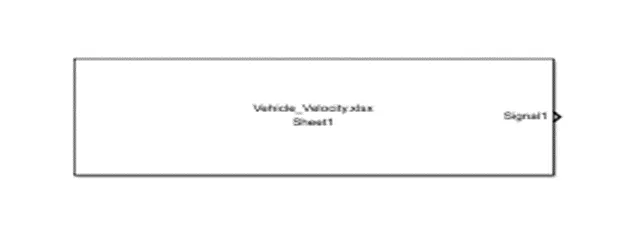
The From Workspace block reads data into a Simulink model from a workspace and provides the data as a signal or a nonvirtual bus at the block's output. You can load data from the base workspace, model workspace, or mask workspace. You can use the From Workspace block to load signal data into any model or subsystem in a model hierarchy from a workspace accessible to the referenced model or subsystem. You can specify how the block constructs the output from the workspace data, including the output sample period, interpolation and extrapolation behavior, and whether to use zero-crossing detection. The From Workspace block icon shows the value of the Data parameter. For example, if you use the From Workspace block to load data in the variable x, you specify x as the value for the Data parameter, and the block displays x.

Specify Data to Load

Specify data for the From Workspace block to load using the Data parameter. You can specify the value of the Data parameter as a MATLAB expression, such as a variable name. The expression in the Data parameter must evaluate to data in a format that the From Workspace block supports. For details about how the expression is evaluated, see Symbol of resolution. The From Workspace block does not load data from a data dictionary. Use a data dictionary to store only design data for a model, not simulation input data. You can store design data related to the From Workspace block, such as the value for the Sample time parameter, in a data dictionary.

Slider Gain:

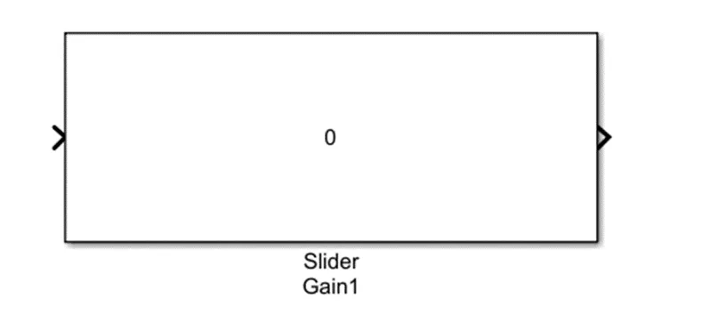
The Slider Gain block performs a scalar gain that you can modify during simulation. Modify the gain using the slider parameter. The Slider Gain block accepts real or complex-valued scalar, vector, or matrix input. The block supports fixed-point data types. The Slider Gain block outputs the input multiplied by a constant gain value. When the input to the block is real and gain is complex, the output is complex

Multiport Switch:

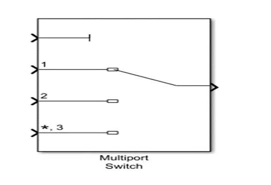
The Multiport Switch block determines which of several inputs to the block passes to the output. The block bases this decision on the value of the first input. The first input is the control input and the remaining inputs are the data inputs. The value of the control input determines which data input passes to the output.The table summarizes how the block interprets the control input and determines the data input that is passed to the output.

Multiport Switch Configured as an Index Vector Block

An Index vector is a special configuration of a Multiport Switch block in which you specify one data input and the control input is zero-based. The block output is the element of the input vector whose index matches the control input. For example, if the input vector is [18 15 17 10] and the control input is 3, the element that matches the index of 3 (zero-based) is 10, and that becomes the output value. To configure a Multiport Switch block to work as an Index Vector block, set Number of data ports to 1 and Data port order to Zero-based contiguous.

How the Block Handles an Out-of-Range Control Input

For an input with an integer value less than intmax(‘int32’), the input is out of range when the value does not match any data port indices. For a control input that is not an integer value, the input is out of range when the truncated value does not match any data port indices. In both cases, the block behavior depends on your settings for Data port for default case and Diagnostic for default case.

 Longitudinal Driver:

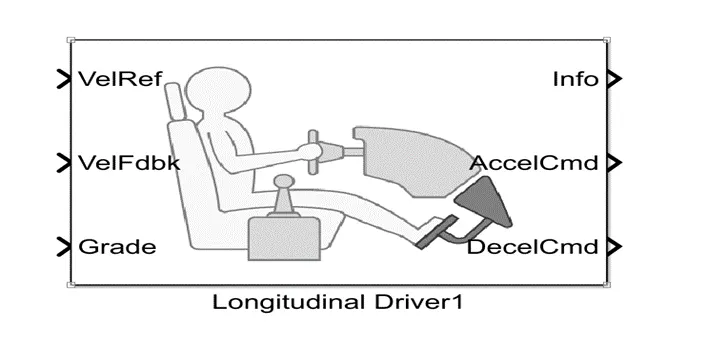
The Longitudinal Driver block implements a longitudinal speed-tracking controller. Based on reference and feedback velocities, the block generates normalized acceleration and braking commands that can vary from 0 through 1. You can use the block to model the dynamic response of a driver or to generate the commands necessary to track a longitudinal drive cycle.

Configurations

Use the External Actions parameters to create input ports for signals that can disable, hold, or override the closed-loop acceleration or deceleration commands. The block uses this priority order for the input commands: disable (highest), hold, override.

This table summarizes the external action parameters.
Goal	External Action Parameter	Input Ports	Data Type
Override the accelerator command with an input acceleration command.	Accelerator override	EnablAccelOvr	Boolean
		AccelOvrCmd	double
Hold the acceleration command at the current value.	Accelerator hold	AccelHld	Boolean
Disable the acceleration command.	Accelerator disable	AccelZero	Boolean
Override the decelerator command with an input deceleration command.	Decelerator override	EnablDecelOvr	Boolean
		DecelOvrCmd	double
Hold the decelerator command at current value.	Decelerator hold	DecelHld	Boolean
Disable the decelerator command.	Decelerator disable	DecelZero	Boolean

Controlled PWM voltage:

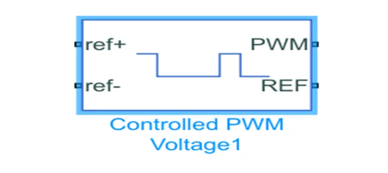
The Controlled PWM Voltage block represents a pulse-width modulated (PWM) voltage source. You can model electrical or physical signal input ports by setting the Modeling option parameter to either:

Electrical input ports — The block calculates the duty cycle based on the reference voltage across its ref+ and ref- ports. This option is the default. PS input — Specify the duty cycle value directly by using an input physical signal port. If you set Modeling option to Electrical input ports, the demanded duty cycle is

100*(Vref-Vmin/Vmax-Vmin)  Percentage

where:

Vref is the reference voltage across the ref+ and ref- ports.

Vmin is the minimum reference voltage.

Vmax is the maximum reference voltage.

Here we are using average PWM frequency is 100Hz and output voltage is 72volts.

The value of the Output voltage amplitude parameter determines amplitude of the output voltage. At time zero, the pulse is initialized as high, unless the Pulse delay time parameter is greater than zero, or the demanded duty cycle is zero. You can use parameters Pulse delay time and Pulse width offset to add a small turn-on delay and a small turn-off advance. This can be useful when fine-tuning switching times so as to minimize switching losses. In PWM mode, the block has two options for the type of switching event when moving between output high and output low states:

Asynchronous – Best for variable-step solvers — Asynchronous events are better suited to variable step solvers, because they require fewer simulation steps for the same level of accuracy. In asynchronous mode the PWM switching events generate zero crossings, and therefore switching times are always determined accurately, regardless of the simulation maximum step size. Discrete—time – Best for fixed-step solvers — Discrete-time events are better suited to fixed-step operation, because then the switching events are always synchronized with the simulation step. Using an asynchronous implementation with fixed-step solvers may sometimes result in events being up to one simulation step late. For more information,

If you use a fixed-step or local solver and the discrete-time switching event type, the following restrictions apply to the Sample time parameter value The sample time must be a multiple of the simulation step size. The sample time must be small compared to the PWM period, to ensure sufficient resolution.

Assumptions and Limitations

The model is based on the following assumptions:

The REF output of this block is floating, it is not tied to the Electrical Reference. One consequence of this is that if you connect the PWM and REF electrical ports directly to the PWM and REF electrical ports of an H-bridge or a gate driver, you must attach an Electrical Reference block to the REF connection line. Do not connect the Controlled PWM block directly to a semiconductor gate, because this omits the gate driver output impedance that determines switching dynamics. Use a Gate Driver or a Half-Bridge Driver block to set the gate-source or the gate-emitter voltage. Do not use the Controlled PWM block to drive a motor block directly. A PWM motor driver goes open circuit in between pulses. Use the H-Bridge block to drive a motor block. When driving a motor via the H-Bridge block, set the Simulation mode parameter to Averaged to speed up simulations. You must also set the Simulation mode parameter of the H-Bridge block to Averaged mode. This applies the average of the embedded PWM voltage to the motor. The Averaged mode assumes that the impedance of the motor inductive term is small at the PWM frequency. To verify this assumption, run the simulation using the PWM mode and compare the results to those obtained from using the Averaged mode. If you are linearizing your model, set the Simulation mode parameter to Averaged and ensure that you have specified the operating point of the block correctly. You can only linearize the block for inputs corresponding to a duty cycle greater than zero and less than 100 percent. When you use this block in PWM mode with the Use local solver option selected in the Solver Configuration block, set the Switching event type parameter to Discrete—time – Best for fixed-step solvers. Using the Asynchronous – Best for variable-step solvers option in this situation may produce inaccuracies, because simulation with the local solver implies fixed step, and the PWM events will not always coincide precisely with the simulation steps. This results in PWM events sometimes occurring one simulation step late.

H-Bridge:

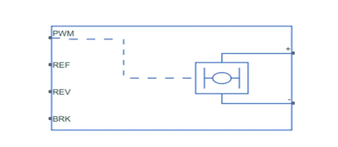
The H-Bridge block represents an H-bridge motor driver. The block has the following two Simulation mode options:

PWM — The H-Bridge block output is a controlled voltage that depends on the input signal at the PWM port. If the input signal has a value greater than the Enable threshold voltage parameter value, the H-Bridge block output is on and has a value equal to the value of the Output voltage amplitude parameter. If it has a value less than the Enable threshold voltage parameter value, the block maintains the load circuit using one of the following three Freewheeling mode options:

Via one semiconductor switch and one freewheeling diode

Via two freewheeling diodes

Via two semiconductor switches and one freewheeling diode

The first and third options are sometimes referred to as synchronous operation.

The signal at the REV port determines the polarity of the output. If the value of the signal at the REV port is less than the value of the Reverse threshold voltage parameter, the output has positive polarity; otherwise, it has negative polarity.

Averaged — This mode has two Load current characteristics options:

Smoothed

Unsmoothed or discontinuous

The Smoothed option assumes that the current is practically continuous due to load inductance. In this case, the H-Bridge block output is:

VoVpwm/Apwm-IoutRon

where:

VO is the value of the Output voltage amplitude parameter.

VPWM is the value of the voltage at the PWM port.

APWM is the value of the PWM signal amplitude parameter.

IOUT is the value of the output current.

RON is the Bridge on resistance parameter.

The current will be smooth if the PWM frequency is large enough. Synchronous operation where freewheeling is via a bridge arm back to the supply also helps smooth the current. For cases where the current is not smooth, or possibly discontinuous (that is, it goes to zero between PWM cycles), use the Unsmoothed or discontinuous option. For this option, you must also provide values for the Total load series resistance, Total load series inductance, and PWM frequency. During simulation, the block uses these values to calculate a more accurate value for H-bridge output voltage that achieves the same average current as would be present if simulating in PWM mode.

Set the Simulation mode parameter to Averaged to speed up simulations when driving the H-Bridge block with a Controlled PWM Voltage block. You must also set the Simulation mode parameter of the Controlled PWM Voltage block to Averaged mode. This applies the average of the demanded PWM voltage to the motor. The accuracy of the Averaged mode simulation results relies on the validity of your assumption about the load current. If you specify that the current is Unsmoothed or discontinuous, then the accuracy also depends on the values you provide for load resistance and inductance being representative. This mode also makes some simplifying assumptions about the underlying equations for the case when current is discontinuous. For typical motor and bridge parameters, accuracy should be within a few percent. To verify Averaged mode accuracy, run the simulation using the PWM mode and compare the results to those obtained from using the Averaged mode.

Braking mode is invoked when the voltage presented at the BRK port is larger than the Braking threshold voltage. Regardless of whether in PWM or Averaged mode, when in braking mode the H-bridge is modeled by a series combination of two resistances R1 and R2 where:

R1 is the resistance of a single bridge arm, that is, half the value of the Total bridge on resistance parameter.

R2 is the resistance of a single bridge arm in parallel with a diode resistance, that is, R1 · Rd / ( R1 + Rd ), where Rd is the diode resistance.

 

External Power Supply

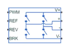
To model the demands placed on the DC supply, you can choose to expose the power supply ports of the H-Bridge block by setting the Power supply parameter to External. If the power supply ports are exposed, then only PWM simulation mode is supported.

Model Thermal Effects

This block has one optional thermal port. To expose the thermal port, set the Modeling option parameter to either:

No thermal port — The block does not contain a thermal port.

Show thermal port — The block contains one thermal conserving port.

When you expose the thermal port:

The heat generated by the bridge on-resistance and freewheeling diodes is added to the thermal port. The thermal port has an associated thermal mass and initial temperature that you can set from the Thermal Port parameters. The bridge on-resistance and freewheeling diode resistance become functions of temperature. You can define the values for these resistances and the second measurement temperature from the Temperature Dependence parameters. Resistance is assumed to vary linearly between the two measurement temperatures. Extrapolation is used for temperatures outside of this range, except for when simulating in averaged mode with discontinuous load current characteristics.

Assumptions and Limitations

If you are linearizing your model, set the Simulation mode parameter to Averaged and ensure that you have specified the operating point correctly. You can only linearize the H-Bridge block for duty cycles that are greater than zero and less than the PWM signal amplitude. If you need to linearize around zero duty cycle, and if your controller always uses regenerative braking mode, set the Regenerative braking parameter to Always enabled (suitable for linearization).

In Averaged mode, and with the Unsmoothed or discontinuous choice for Load current characteristics, you must provide representative values for load inductance and resistance. If driving a DC Motor, then the resistance is the armature resistance, and the inductance is the sum of the armature inductance plus series smoothing inductor (if present). For a Universal Motor, total resistance is the sum of the armature and field windings, and total inductance is the sum of armature and field inductances plus any series smoothing inductance. For a Shunt Motor, MathWorks recommends that you draw a Thévenin equivalent circuit to determine appropriate values. No forward voltage is modeled for the freewheeling diodes. They are approximated as ideal resistances when forward biased, with resistance equal to the Freewheeling diode on resistance parameter value.

If the supply rail connections are exposed, only the PWM simulation mode is supported.

DC motor:

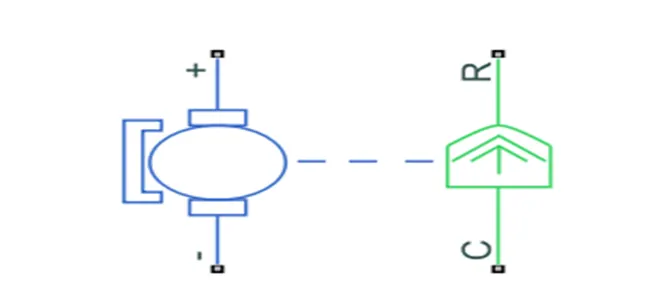
The DC Motor block represents the electrical and torque characteristics of a DC motor using the following equivalent circuit model:

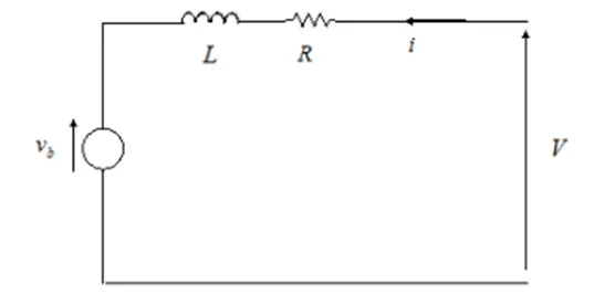
You specify the equivalent circuit parameters for this model when you set the Model parameterization parameter to By equivalent circuit parameters. The resistor R corresponds to the resistance you specify in the Armature resistance parameter. The inductor L corresponds to the inductance you specify in the Armature inductance parameter. You can specify how to generate the magnetic field of the DC motor by setting the Field type parameter to the desired option.

Here we are using parmanent magnet DC motor of by rated load and speed

parameters using for Parmanent magnet DC motor is

Rated supply voltage = 72v DC

Rated mechanical Power = 130Kw

Rated Speed is 2500 rpm and

No load speed is 3000 rpm

Armature inductance is 12e-6 Hendries

The permanent magnets in the motor induce the following back emf vb in the armature:

vb=kvω

where kv is the Back-emf constant and ω is the angular velocity. The motor produces the following torque, which is proportional to the motor current i:

TE=kti

where kt is the Torque constant. The DC Motor block assumes that there are no electromagnetic losses. This means that mechanical power is equal to the electrical power dissipated by the back emf in the armature. Equating these two terms gives:

TEω=vbiktiω=kvωikv=kt

As a result, you specify either kv or kt in the block parameters.

If the magnetic field is generated from the current flowing through the windings, the Back-emf constant depends on the field current If:

kv=LafIf

where Laf is the Field-armature mutual inductance.

The torque-speed characteristic for the DC Motor block is related to the parameters in the preceding figure. When you set the Model parameterization parameter to By stall torque & no-load speed or By rated power, rated speed & no-load speed, the block solves for the equivalent circuit parameters as follows:

For the steady-state torque-speed relationship, L has no effect.

Sum the voltages around the loop and rearrange for i:

I=(V-Vb/R)=(V-kvw/R)

Substitute this value of i into the equation for torque:

TE=((kt/R)V-kvw)

When you set the Model parameterization parameter to By stall torque & no-load speed, the block uses the stall torque and no-load speed to determine values for R and kt (and equivalently kv). When you set the Model parameterization parameter to By rated power, rated speed & no-load speed, the block uses the rated speed and power to calculate the rated torque. The block uses the rated torque and no-load speed values to determine values for R and kt.

The block models motor inertia J and damping λ for all values of the Model parameterization parameter. The resulting torque across the block is:

TE=((kt/R)V-kvw)-Jw-‘lamda’w

It is not always possible to measure rotor damping, and rotor damping is not always provided on a manufacturer datasheet. An alternative is to use the no-load current to infer a value for rotor damping.

For no-load, the electrically-generated mechanical torque must equal the rotor damping torque:

ktinoload=λωnoload

where in no load is the no-load current. If you select by no-load current for the Rotor damping parameterization parameter, then this equation is used in addition to the torque-speed equation to determine values for λ and the other equation coefficients. The value for rotor damping, whether specified directly or in terms of no-load current, is taken into account when determining equivalent circuit parameters for Model parameterization options By stall torque and no-load speed and By rated power, rated speed and no-load speed. When a positive current flows from the electrical + to - ports, a positive torque acts from the mechanical C to R ports.

Faults

The DC Motor block allows you to model two types of faults:

Armature winding fault — The armature winding fails and goes open circuit.

Field winding fault — The field winding that creates the magnetic field fails and goes open circuit.

The block can trigger fault events:

At a specific time (temporal fault).

When a current limit is exceeded for longer than a specific time interval (behavioral fault). You can enable or disable these trigger mechanisms separately. You can choose whether to issue an assertion when a fault occurs, by using the Reporting when a fault occurs parameter. The assertion can take the form of a warning or an error. By default, the block does not issue an assertion.

This figure shows a generic representation of a DC motor, with brushes, armatures, commutators, and their windings:

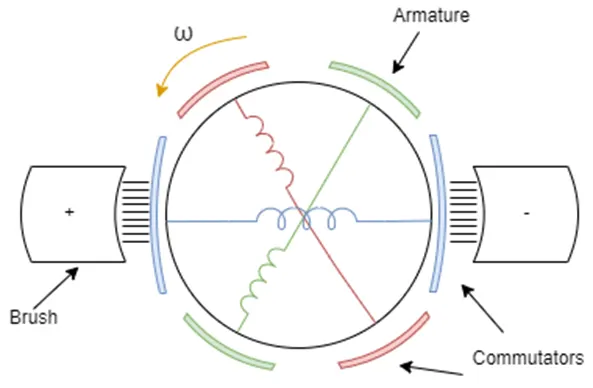
If you set the Enable armature winding open-circuit fault parameter to On, the armature fails at the time specified by the Simulation time for armature winding fault event parameter for a temporal fault, or when the winding currents exceeds the value of the Maximum permissible armature winding current parameter for a behavioral fault. When the armature fails, the voltage source connected to this block observes an open circuit for a fraction of the total motor revolution, specified by the Fraction of revolution during which armature is open-circuit parameter, rev_faulted. This figure illustrates the circuit state behavior for a certain rev_faulted during the entire revolution period:

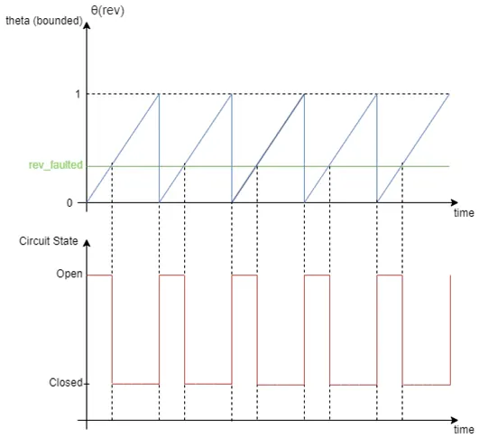
Predefined Parameterization

There are multiple available built-in parameterizations for the permanent magnet DC Motor block. This pre-parameterization data allows you to set up the block to represent components by specific suppliers. The parameterizations of these DC motors match the manufacturer data sheets. To load a predefined parameterization, double-click the DC Motor block, click the  hyperlink of the Selected part parameter and, in the Block Parameterization Manager window, select the part you want to use from the list of available components.

Model Thermal Effects

You can expose the thermal port to model the effects of losses that convert power to heat. To expose the thermal port, set the Modeling option parameter to either:

No thermal port — The block does not contain a thermal port.

Show thermal port — The block contains one thermal conserving port.

Vehicle Body:

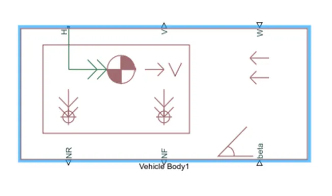
The Vehicle Body block represents a two-axle vehicle body in longitudinal motion. The vehicle can have the same or a different number of wheels on each axle. For example, two wheels on the front axle and one wheel on the rear axle. The vehicle wheels are assumed identical in size. The vehicle can also have a center of gravity (CG) that is at or below the plane of travel. The block accounts for body mass, aerodynamic drag, road incline, and weight distribution between axles due to acceleration and road profile. Optionally include pitch and suspension dynamics. The vehicle does not move vertically relative to the ground. The block has an option to include an externally-defined mass and an externally-defined inertia. The mass, inertia, and center of gravity of the vehicle body can vary over the course of simulation in response to system changes.

Model

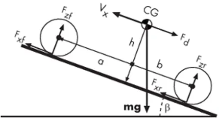
The vehicle axles are parallel and form a plane. The longitudinal, x, direction lies in this plane and perpendicular to the axles. If the vehicle is traveling on an incline slope, β, the normal, z, direction is not parallel to gravity but is always perpendicular to the axle-longitudinal plane.

This figure and table define the vehicle motion model variables.

Vehicle Dynamics and Motion

 

Equations

Vehicle Dynamics

The vehicle motion is a result of the net effect of all the forces and torques acting on it. The longitudinal tire forces push the vehicle forward or backward. The weight mg of the vehicle acts through its center of gravity (CG). Depending on the incline angle, the weight pulls the vehicle to the ground and pulls it either backward or forward. Whether the vehicle travels forward or backward, aerodynamic drag slows it down. For simplicity, the drag is assumed to act through the CG.

m˙Vx=Fx−​ Fd−mg⋅sinβ 

Fx=n(Fxf+Fxr) 

Fd=(1/2)CdρA(Vx+Vw)2⋅sgn(Vx+Vw)

Zero normal acceleration and zero pitch torque determine the normal force on each front and rear wheel.

Fzf=(-h(Fd+ mg⋅sinβ+ m˙Vx) +b⋅mgcosβ)/ n(a+b)

Fzr=( +h(Fd+mgsinβ+m˙Vx)+b⋅mgcosβ)/ n(a+b)

The wheel normal forces satisfy Fzf+Fzr=mg(cosβ/n).

If you include an externally-defined mass or inertia, the equations are shifted by the weighted value of the input.

Pitch dynamics

Pitch acceleration depends on three torque components and the inertia of the vehicle:

α= (f⋅h)+(Fzfa)−(Fzrb)/J

Where:

ɑ is the pitch acceleration.

f is the longitudinal force.

h is the height of the center of gravity when measured parallel to the z-axis.

J is the inertia.

If you choose a linear model for suspension stiffness and damping, the block uses small angle approximation for pitch calculations. If you choose a table lookup model, the block uses the vectors that you specify calculate pitch dynamics. For hard stop equations.

Variables

To set the priority and initial target values for the block variables prior to simulation, use the Initial Targets section in the block dialog box or Property Inspector. For more information. Nominal values provide a way to specify the expected magnitude of a variable in a model. Using system scaling based on nominal values increases the simulation robustness. Nominal values can come from different sources, one of which is the Nominal Values section in the block dialog box or Property Inspector. For more information.

Limitations and Assumptions

The Vehicle Body block lets you model only longitudinal dynamics, parallel to the ground and oriented along the direction of motion. The vehicle is assumed to be in pitch and normal equilibrium. The block does not model pitch or vertical movement. As such, the equations assume that the wheels never lose contact. This constraint can result in negative normal forces.

Tire:

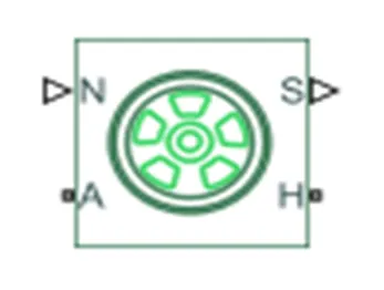
The Tire (Magic Formula) block represents a tire with longitudinal behavior given by the Magic Formula [1], an empirical equation based on four fitting coefficients. The block can model tire dynamics under constant or variable pavement conditions. The longitudinal direction of the tire is the same as its direction of motion as it rolls on pavement. This block is a structural component based on the Tire-Road Interaction (Magic Formula) block. To increase the fidelity of the tire model, you can specify properties such as tire compliance, inertia, and rolling resistance. However, these properties increase the complexity of the tire model and can slow down simulation. Consider ignoring tire compliance and inertia if simulating the model in real time or if preparing the model for hardware-in-the-loop (HIL) simulation.

Tire Model

The Tire (Magic Formula) block models the tire as a rigid wheel-tire combination in contact with the road and subject to slip. When torque is applied to the wheel axle, the tire pushes on the ground (while subject to contact friction) and transfers the resulting reaction as a force back on the wheel. This action pushes the wheel forward or backward. If you include the optional tire compliance, the tire also flexibly deforms under load.

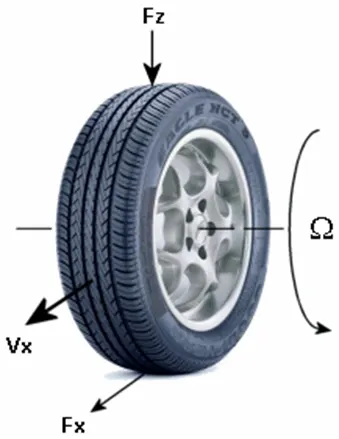
The figure shows the forces acting on the tire. The table defines the tire model variables.

Tire Kinematics and Response

Roll and Slip

The equation for translational motion of a non-slipping, non-compliant tire is Vx=rwΩ. When tires experience slip, they respond by developing a longitudinal force, Fx.

The contact patch slip velocity is V′sx=rwΩ+˙u−Vx. For a tire without compliance, u = 0. The block defines the contact patch slip as

k′= (V′sx/ √V2th+V2x,

where the square root expression provides numerical robustness when Vx = 0. For example, in the case of a non-translating, spinning tire, Vx=0 while k=( rwΩ)/ Vth is finite.

When the tire deformation is negligible and the wheel hub longitudinal velocity is sufficiently large, the equation for wheel slip approaches

k=( Vsx/ ∣Vx∣).

For this equation, a locked, sliding wheel has k = -1. For perfect rolling, k = 0.

Deformation

If the tire is modeled with compliance, it is also flexible. In this case, because the tire deforms, the tire-road contact point turns at a slightly different angular velocity, Ω′, from the wheel, Ω, and requires, instead of the wheel slip, the contact point or contact patch slip κ'. The block models the deforming tire as a translational spring-damper of stiffness, CFx, and damping, bFx.

If you model a tire without compliance, that is, if u=0, then there is no tire longitudinal deformation at any time in the simulation and:

k′=k

V′sx=Vsx

Ω′=Ω

Tire and Wheel Dynamics

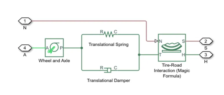
The full tire model is equivalent to this Simscape™/Simscape Driveline™ component diagram. It simulates both transient and steady-state behavior and correctly represents starting from, and coming to, a stop. The Translational Spring and Translational Damper are equivalent to the tire stiffness CFx and damping bFx. The Tire-Road Interaction (Magic Formula) block models the longitudinal force Fx on the tire as a function of Fz, and k′ using the Magic Formula, with k′ as the independent slip variable. Here, Fz is the input signal at port N. The Wheel and Axle radius is the tire rolling radius rw. The Mass value is the effective mass, Iwr2w. The tire characteristic function f(k′, Fz) determines the longitudinal force Fx. Together with the driveshaft torque applied to the wheel axis, Fx determines the wheel angular motion and longitudinal motion.

Without tire compliance, the Translational Spring and Translational Damper are omitted, and contact variables revert to wheel variables. In this case, the tire effectively has infinite stiffness, and port P of Wheel and Axle connects directly to port T of Tire-Road Interaction (Magic Formula).

Without tire inertia, the Mass is omitted.

Assumptions and Limitations

The Tire (Magic Formula) block assumes longitudinal motion only and includes no camber, turning, or lateral motion. Tire compliance implies a time lag in the tire response to the forces on it. Time lag simulation increases model fidelity but reduces simulation performance.

Battery:

   

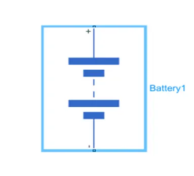
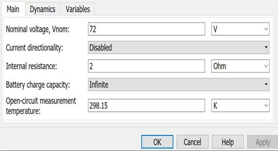
The Battery block represents a simple battery model. The block has four modeling options, accessible by setting the Modeling option parameter to either:

Uninstrumented | No thermal port — Basic model that does not output battery charge level or simulate thermal effects.

Uninstrumented | Show thermal port — Model with exposed thermal port. This model does not measure internal charge level of the battery.

Instrumented | No thermal port — Model with exposed charge output port. This model does not simulate thermal effects.

Instrumented | Show thermal port — Model that lets you measure internal charge level of the battery and simulate thermal effects. Both the thermal port and the charge output port are exposed.

The instrumented modeling options have an extra physical signal port that outputs the internal state of charge. Use this functionality to change load behavior as a function of state of charge, without the complexity of building a charge state estimator.

The thermal port modeling options expose a thermal port, which represents the battery thermal mass. When you select this option, provide additional parameters to define battery behavior at a second temperature. For more information.

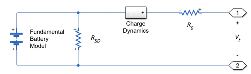
The battery equivalent circuit is made up of the fundamental battery model, the self-discharge resistance RSD, the charge dynamics model, and the series resistance R0.

Battery Model

If you select Infinite for the Battery charge capacity parameter, the block models the battery as a series resistor and a constant voltage source. If you select Finite for the Battery charge capacity parameter, the block models the battery as a series resistor and a charge-dependent voltage source. In the finite case, the voltage is a function of charge and has the following relationship:

V=V0((SOC)/ 1−β(1−SOC))

where:

SOC (state-of-charge) is the ratio of current charge to rated battery capacity.

V0 is the voltage when the battery is fully charged at no load, as defined by the Nominal voltage, Vnom parameter. β is a constant that is calculated so that the battery voltage is V1 when the charge is AH1.

Specify the voltage V1 and cell capacityAH1 using block parameters. AH1 is the charge when the no-load (open-circuit) voltage is V1, and V1 is less than the nominal voltage. The equation defines an approximate relationship between voltage and remaining charge. This approximation replicates the increasing rate of voltage drop at low charge values, and ensures that the battery voltage becomes zero when the charge level is zero. The advantage of this model is that it requires few parameters, which are readily available on most datasheets.

Modeling Battery Fade

For battery models with finite battery charge capacity, you can model battery performance deterioration depending on the number of discharge cycles. This deterioration is referred to as battery fade. To enable battery fade, set the Battery fade parameter to Enabled. This setting exposes additional parameters in the Fade section. The block implements battery fade by scaling certain battery parameter values that you specify in the Main section, depending on the number of completed discharge cycles. The block uses multipliers λAH, λR0, and λV1 on the Cell capacity (Ah rating), Internal resistance, and Voltage V1 when charge is AH1 parameter values, respectively. These multipliers, in turn, depend on the number of discharge cycles:

λAH=1−k1N0.5

λR0=1+k2N0.5

λV1=1−k3N

`N=(N0+1/(Ah)int 0toti(t).H(i(t)))/(lamdaAh(t))`

where:

λAH is the multiplier for battery nominal capacity.

λR0 is the multiplier for battery series resistance.

λV1 is the multiplier for voltage V1.

N is the number of discharge cycles completed.

N0 is the number of full discharge cycles completed before the start of the simulation.

AH is the rated battery capacity in ampere-hours.

i(t) is the instantaneous battery output current.

H(i(t)) is the Heaviside function of the instantaneous battery output current. This function returns 0 if the argument is negative, and 1 if the argument is positive.

The block calculates the coefficients k1, k2, and k3 by substituting the parameter values you provide in the Fade section into these battery equations. For example, the default set of block parameters corresponds to the following coefficient values:

k1 = 1e-2

k2 = 1e-3

k3 = 1e-3

You can also define a starting point for a simulation based on the previous charge-discharge history by using the high-priority variable Discharge cycles. For more information.

Modeling Thermal Effects

If you set the Modeling option parameter to either Uninstrumented | Show thermal port or Instrumented | Show thermal port, you provide additional parameters to define battery behavior at a second temperature. The extended equations for the voltage when the thermal port is exposed are:

V=V0T((SOC)/ 1−βT(1−SOC))

V0T=V0(1+λV(T−T1))

where:

T is the battery temperature.

T1 is the nominal measurement temperature.

λV is the parameter temperature dependence coefficient for V0.

βT=β[1+λβ(T−T1)].

λβ is the parameter temperature dependence coefficient for β.

β is calculated in the same way as battery model, using the temperature-modified nominal voltage V0T.

The internal series resistance, self-discharge resistance, and any charge-dynamic resistances are also functions of temperature:

RT=R(1+λR(T−T1))

where λR is the parameter temperature dependence coefficient.

All the temperature dependence coefficients are determined from the corresponding values you provide at the nominal and second measurement temperatures. If you include charge dynamics in the model, the time constants vary with temperature in the same way.

The battery temperature is determined from a summation of all the ohmic losses included in the model:

 `MthT=isum(VT.i^2)/(RT.i)`

where:

Mth is the battery thermal mass.

i corresponds to the ith ohmic loss contributor. Depending on how you have configured the block, the losses include:

Series resistance

Self-discharge resistance

First charge dynamics segment

Second charge dynamics segment

Third charge dynamics segment

Fourth charge dynamics segment

Fifth charge dynamics segment

VT,i is the voltage drop across resistor i.

RT,i is resistor i.

Modeling Charge Dynamics

You can model battery charge dynamics using the Charge dynamics parameter:

No dynamics — The equivalent circuit contains no parallel RC sections. There is no delay between terminal voltage and internal charging voltage of the battery.

One time-constant dynamics — The equivalent circuit contains one parallel RC section. Specify the time constant using the First time constant parameter.

Two time-constant dynamics — The equivalent circuit contains two parallel RC sections. Specify the time constants using the First time constant and Second time constant parameters.

Three time-constant dynamics — The equivalent circuit contains three parallel RC sections. Specify the time constants using the First time constant, Second time constant, and Third time constant parameters.

Four time-constant dynamics — The equivalent circuit contains four parallel RC sections. Specify the time constants using the First time constant, Second time constant, Third time constant, and Fourth time constant parameters.

Five time-constant dynamics — The equivalent circuit contains five parallel RC sections. Specify the time constants using the First time constant, Second time constant, Third time constant, Fourth time constant, and Fifth time constant parameters.

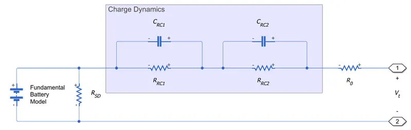
 This figure shows the equivalent circuit for the block configured with two time-constant dynamics.

In the diagram:

RRC1 and RRC2 are the parallel RC resistances. Specify these values with the First polarization resistance and Second polarization resistance parameters, respectively.

CRC1 and CRC2 are the parallel RC capacitances. The time constant τ for each parallel section relates the R and C values using the relationship C=τ/R. Specify τ for each section using the First time constant and Second time constant parameters, respectively.

R0 is the series resistance. Specify this value with the Internal resistance parameter.

Modeling Battery Aging

For battery models with finite battery charge capacity, you can model the battery performance deterioration that occurs when the battery is not used. Calendar aging affects both the internal resistance and capacity. In particular, the resistance increase depends by various mechanisms such as the creation of Solid Electrolyte Interface (SEI) at both anode and cathode and the corrosion of the current collector. These processes mainly depends on the storage temperature, the storage state of charge, and time.

This equation defines the terminal resistance increase of the battery due to calendar aging:

αr(T,Voc)R=(bVoc−c)e−(qd/kT)

`R=R0(1+lim_(i->oo) sum_(i=1)^Nalphar(Ti,Voc)(T^ai-t^ai-1))`

 where:

Voc is the Normalized open-circuit voltage during storage, V/Vnom.

R0 is the Internal resistance.

ti is the time sample derived from the Vector of time intervals parameter.

Ti is derived from the Vector of temperatures parameter.

b is the Linear scaling for voltage, b.

c is the Constant offset for voltage, c.

d is the Temperature-dependent exponential increase, d.

a is the Time exponent, a.

q is the electron's elementary charge, in C.

k is the Boltzmann constant, in J/K.

The R1_age_multiplier variable in the Simscape Results Explorer stores the calendar aging of the battery in terms of resistance increase:

R1_age_multiplier=R/R0.

For thermal modeling options of the block, if you set the Storage condition parameter to Fixed open-circuit voltage, you must specify the additional Open-circuit voltage measurement temperature parameter to convert the storage open-circuit voltage to the temperature-independent state of charge during storage:

SOC=(OCV(1−β(TOCVmeasurement))/ 1−β(TOCVmeasurement)OCV

The open-circuit voltage according to the storage temperature is then defined by this equation:

SOC=SOC/ 1−β(Tstorage)(1−β(Tstorage)SOC)

Finally, this equation defines the terminal resistance increase of the battery due to calendar aging according to the storage temperature:

Plotting Voltage-Charge Characteristics

A quick plot feature lets you visualize the voltage-charge characteristic for the battery model parameter values. To plot the characteristics, right-click a Battery block in your model and, from the context menu, select Electrical > Basic characteristic. The software automatically computes a set of bias conditions, based on the block parameter values, and opens a figure window containing a plot of no-load voltage versus the state-of-charge (SOC) for the block. For more information,

Variables

To set the priority and initial target values for the block variables prior to simulation, use the Initial Targets section in the block dialog box or Property Inspector. For more information. Nominal values provide a way to specify the expected magnitude of a variable in a model. Using system scaling based on nominal values increases the simulation robustness. Nominal values can come from different sources, one of which is the Nominal Values section in the block dialog box or Property Inspector. For more information. When you model battery fade, the Discharge cycles variable lets you specify the number of charge-discharge cycles completed prior to the start of simulation. If you disable battery fade modeling, this variable is not used by the block.

Assumptions and Limitations

The self-discharge resistance is assumed not to depend strongly on the number of discharge cycles. For the thermal modeling option of the battery, you provide fade data only for the reference temperature operation. The block applies the same derived λAH, λR0, and λV1 multipliers to parameter values corresponding to the second temperature.

When using the thermal block modeling options, use caution when operating at temperatures outside of the temperature range bounded by the Measurement temperature and Second measurement temperature values. The block uses linear interpolation for the derived equation coefficients, and simulation results can become nonphysical outside of the specified range. The block checks that the internal series resistance, self-discharge resistance, and nominal voltage always remain positive. If there is a violation, the block issues error messages.

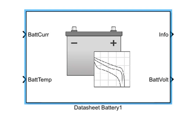
Data sheet Battery:

The Datasheet Battery block implements a lithium-ion, lithium-polymer, or lead-acid battery that you can parameterize using manufacturer data. To create the open-circuit voltage and internal resistance parameters that you need for the block, use the manufacturer discharge characteristics by temperature data. To determine the battery output voltage, the block uses lookup tables for the battery open-circuit voltage and the internal resistance. The lookup tables are functions of the state-of charge (SOC) and battery temperature, characterizing the battery performance at various operating points:

Em=f(SOC)Rint=f(T,SOC)

Model Simulation:

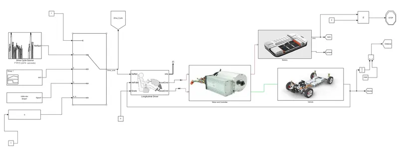
Here Im using 72KW battery pack  which cancapable to deliver 72V and 100Ah power. Permanent magnet DC motor is used for propulsion for Electric vehicke which is runs at 3000 rpm at noload and 2500rpm at full load speeds with 130KW Rated load capacity can handled. To control the motor H brige type PWM controller is used to convert DC supply to pulsating DC supply and Vehicle body used to get rated velocity and Speed to the tire for transimition with respect to wind force, Grading angle and Acceleration give by the Driver. Here Simple Gear used to transmit rational accelaration power to required rotational and Longitudinal Driver used to take Drive cycle as reference velocity and  takes feedback velocity form the Vehicle and gives the acceleration command as required to drive the vehicle.

Scenario 1:

Using FTP75 Drive cycle source:

I'm Taking FTP75 Drive cycle as a reference input velocity and remaining the all other parameters as above discused. Now I'm going to run for 2474 seconds to know by this time my vehicle can travel how much distance and at what time my SOC is dropped from 100 to some percentage. And to know the is my vehicle is running with respect to given drive cycle

Output:

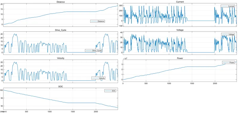
Now run the simulation and observe the simulated results.

Observations:

My EV is travelled 19.47Km and State of charge remained is 89%. for to rrech 19.47Km with 25m/s of peak velocity which is almost near to my drive cycle velocity as given. My vehicle consumed 11% of SOC and Power consumed by the Vehicle is 35 Watts.

Scenario 2:

Wide open Throttle

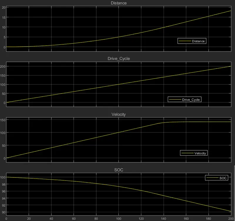
I'm going to give maximum throttle to know the time taken by the vehicle to reach maximum speed of 100 Kmph. And power consumed by the vehicle. For that I'm running the vehicle for 100 sec using Signal Builder block

Output:

Observation:

From the above simulated output graph we can see that when open wide throttle given to the vehicle, it is took 140 sec to reach maximum speed of 140Kmph and battry drainde from 100 to 90 percentage whichnis vehicle consumed 10 percentage of battery.

Scenario 3:

Maximum distace travelled.

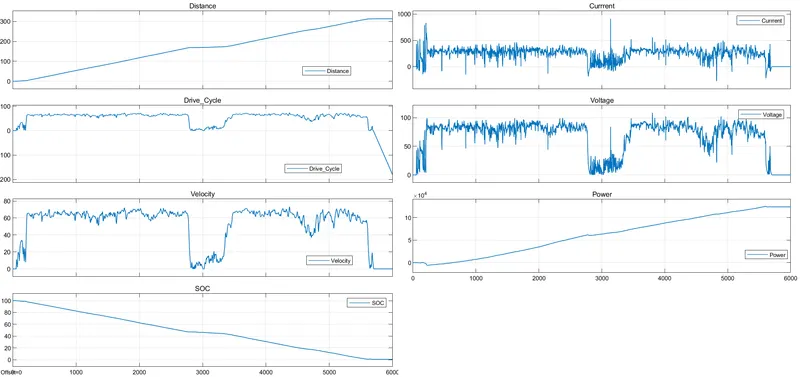
To find out the maximum distance travelled by the vehicle, I'm going discharge the complete battey from 100 to 0 percentage. and amout of power consumed by the vehicle.

Output:

Observation:

Here im taking a drive cycle by using excel by from speadsheet, now this model vehice battery drained from 100 to 0%. vehicle travelled 310Km from starting and power consumed by the vehicle is 126KW. 

Conclusion:

• Obtained to know the battery stateof charge, power consumed by the vehicle and vehicle is travelled nearby same velocity as given by Drive cycle using FTPdrive cycle,
• Otained time taken by the vehicle to reach its maximum speed, we can able set our own drive cycle using slider gain block to know the status of the vehicle.