Final Project: Design of an Electric Vehicle
Create a MATLAB model of an electric car that uses a battery and a DC motor. Choose suitable blocks from the Powertrain block set. Prepare a report about your model including the following:
Objectives:
- System-level configurations
- Model parameters
- Results
- Conclusion
AIM:
The main aim of this project is to create a MATLAB model of the Electric Car with simple and low run time. By using the DC Motor, Battery, and individual component blocks. In this project, the Electric Car’s performance is checked with various Drive Cycles. And check out the Speed of the vehicle, SOC of Battery, Current, and Voltage. To know the Developed MATLAB model and its configuration to match the actual vehicle.
What is EV technology?
Let's start by considering the legacy vehicle technology: the internal combustion engine, or ICE. This vehicle is propelled by a combustion engine that can only be fueled by gasoline. The technology is conventional, well-established, and reliable, but it consumes large amounts of gasoline—which can be costly in many ways.
ICE Vehicle model is shown below figure:
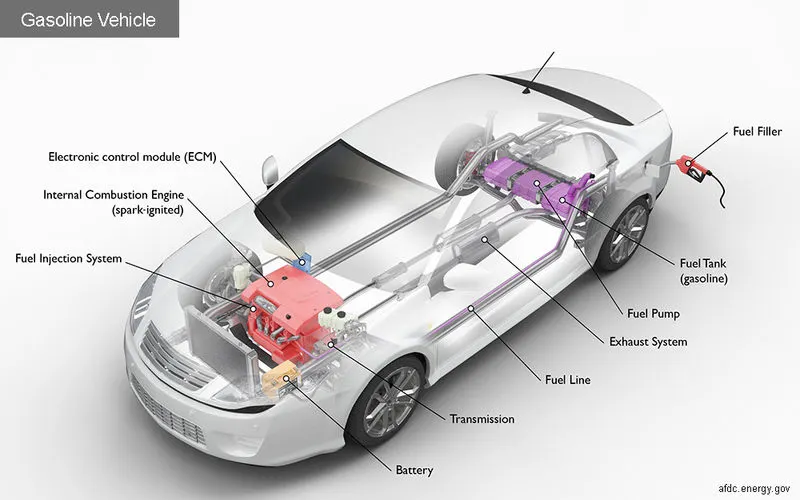
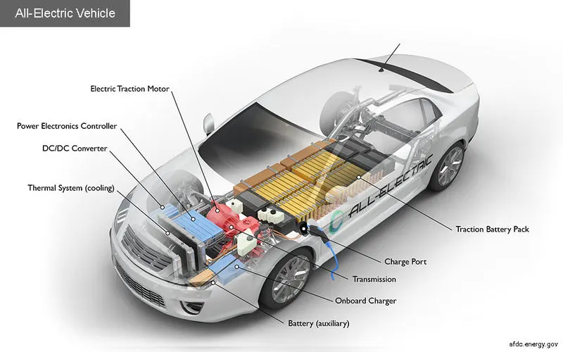
Enter the electric vehicle Unlike internal combustion technology—which uses combustion and pressure to propel a vehicle—electric vehicles, or EVs, are propelled by electromagnetism. These vehicles use electricity, typically stored in a battery, to power an electric motor.
The electric vehicle model is shown below figure:
Types of EV:
There are four types of electric vehicles available:
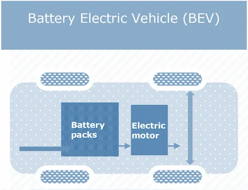
- Battery Electric Vehicle (BEV): Fully powered by electricity. These are more efficient compared to hybrid and plug-in hybrids.
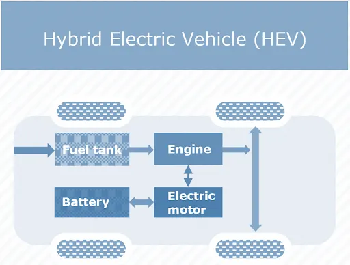
- Hybrid Electric Vehicle (HEV): The vehicle uses both the internal combustion (usual petrol) engine and the battery-powered motor powertrain. The petrol engine is used both to drive and charge when the battery is empty. These vehicles are not as efficient as fully electric or plug-in hybrid vehicles.
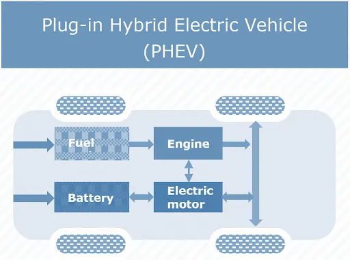
- Plug-in Hybrid Electric Vehicle (PHEV): Uses both an internal combustion engine and a battery charged from an external socket (they have a plug). This means the vehicle’s battery can be charged with electricity rather than the engine. PHEVs are more efficient than HEVs but less efficient than BEVs.
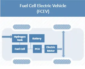
- Fuel Cell Electric Vehicle (FCEV): Electric energy is produced from chemical energy. For example, a hydrogen FCEV.
What are the main components of EV?
Electric vehicles consist of an electric motor that is powered by a battery pack. The main advantage of electric vehicles is that they emit zero emissions and are eco-friendly. They also do not consume any fossil fuels, hence using a sustainable form of energy for powering the car. The main components of electric vehicles are:
- Traction battery pack
- DC-DC Converter
- Electric motor
- Power inverter
- Charge Port
- Onboard charger
- Controller
- Auxiliary batteries
- Thermal system (cooling)
- Transmission
1. Traction battery pack
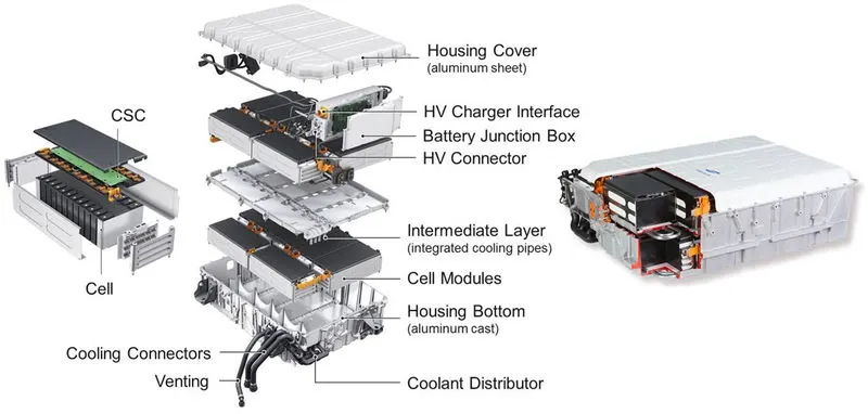
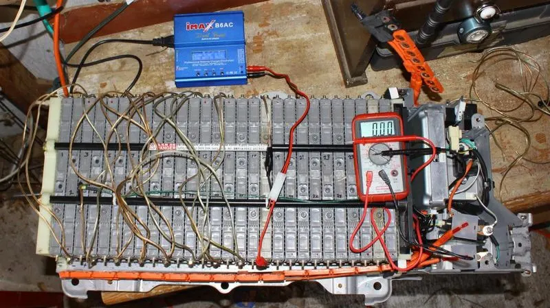
The traction battery pack is also known as an Electric vehicle battery (EVB). It powers the electric motors of an electric vehicle. The battery acts as an electrical storage system. It stores energy in the form of DC current. The range will be higher with increasing kW of the battery. The life and operation of the battery depending on its design. The lifetime of a traction battery pack is estimated to be 200,000 miles.
2. DC-DC Converter:
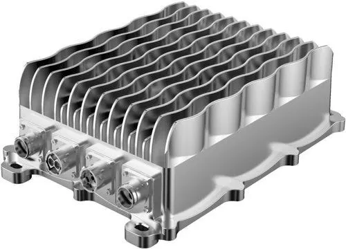
The traction battery pack delivers a constant voltage. But different components of the vehicle have different requirements. The DC-DC converter distributes the output power that is coming from the battery to a required level. It also provides the voltage required to charge the auxiliary battery.
3. Electric motor
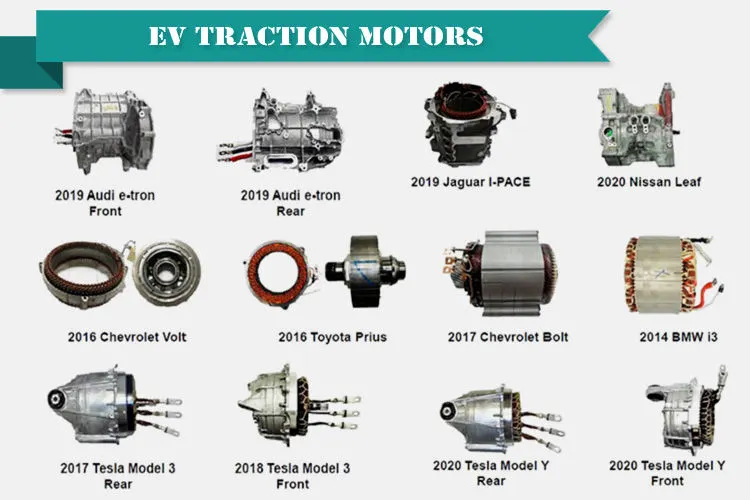
The electric traction motor is the main component of an electric vehicle. The motor converts the electrical energy into kinetic energy. This energy rotates the wheels. The electric motor is the main component that differentiates an electric car from a conventional car. An important feature of an electric motor is the regenerative braking mechanism. This mechanism slows down the vehicle by converting its kinetic energy into another form and storing it for future use. There are basically two types of motors DC and AC motors.
4. Power Inverter
It covers DC power from the batteries to AC power. It also converts the AC current generated during regenerative braking into DC current. This is further used to recharge the batteries.
5. Charge Port
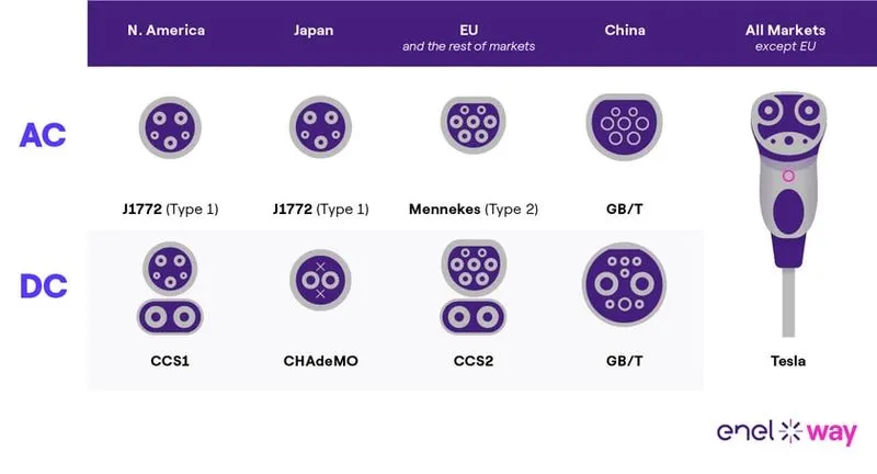
The charge port connects the electric vehicle to an external supply. It charges the battery pack. The charge port is sometimes located in the front or rear part of the vehicle
6. Onboard charger
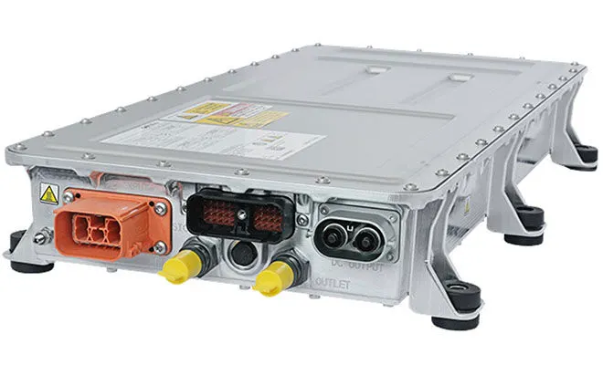
An onboard charger is used to convert the AC supply received from the charge port to the DC supply. The onboard charger is located and installed inside the car. It monitors various battery characteristics and controls the current flowing inside the battery pack.
7. Controller
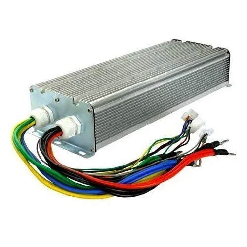
The power electronics controller determines the working of an electric car. It performs the regulation of electrical energy from the batteries to the electric motors. The pedal set by the driver determines the speed of the car and the frequency of variation of voltage that is input to the motor. It also controls the torque produced.
8. Auxiliary batteries
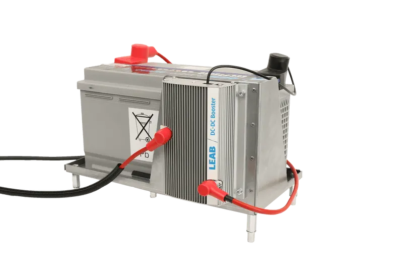
Auxiliary batteries are the source of electrical energy for the accessories in electric vehicles. In the absence of the main battery, the auxiliary batteries will continue to charge the car. It prevents the voltage drop, produced during engine start from affecting the electrical system.
9. Thermal system(cooling)
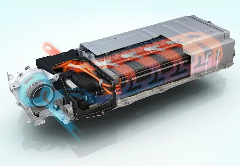
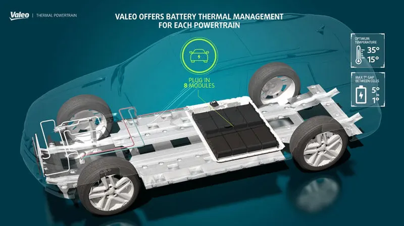
The thermal management system is responsible for maintaining an operating temperature for the main components of an electric vehicle such as an electric motor, controller, etc. It functions during charging as well to obtain maximum performance. It uses a combination of thermoelectric cooling, forced air cooling, and liquid cooling.
10. Transmission
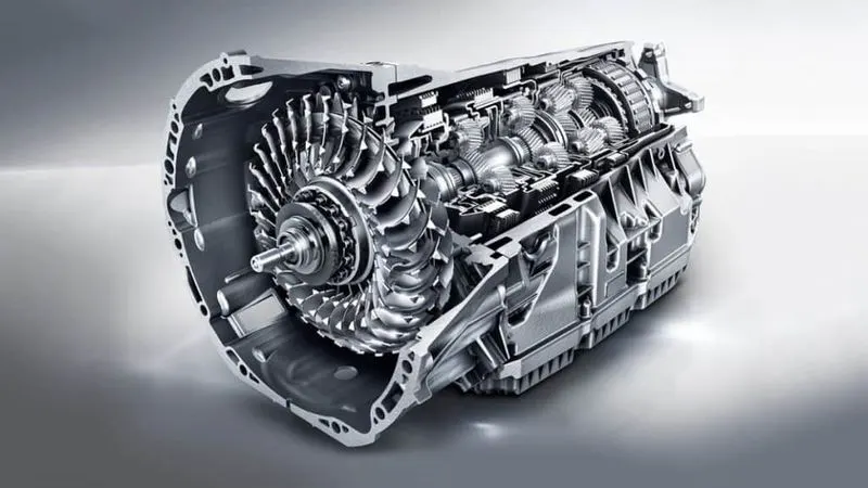
It is used to transfer the mechanical power from the electric motor to the wheels, through a gearbox. The advantage of electric cars is that they do not require multi-speed transmissions. The transmission efficiency should be high to avoid power loss.
Block Diagram of EV:
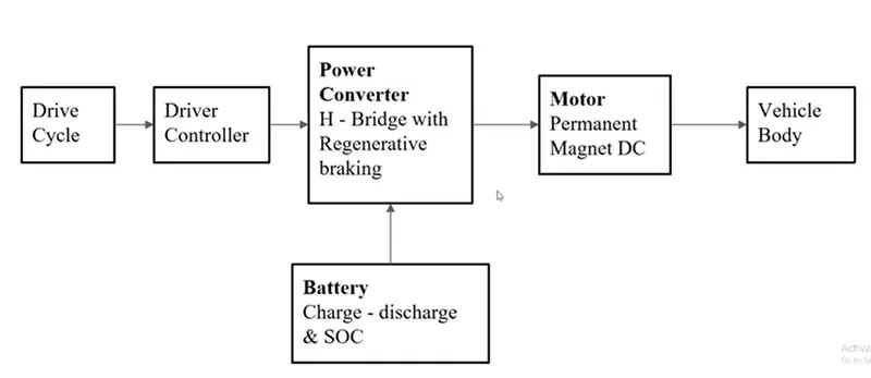
The block diagram shows the arrangement of the components of the electric vehicle.
The Drive cycle has used the input of the driver controller. The driver controller controls the Acceleration and Braking of the power converter. The power converter H- Bridge is having a regenerative braking system. The DC motor is driven by the H-Bridge power converter. DC motor is connected to the vehicle body block. This block consists of vehicle transmission components like gear, wheels, and vehicle body. Finally, the battery is connected to the power converter block. This block consists of battery parameters charge, discharge, and SOC. The driver controller block has velocity feedback from the vehicle body to control the power converter. The motor block has the DC Motor and mechanical connection blocks.
MATLAB model:
The MATLAB modeling of an Electric Car by using the DC motor, Battery and choosing the suitable blocks from the powertrain block set is developed and shown below.
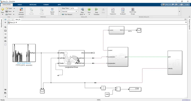
The MATLAB model is designed and arranged the blocks according to the block diagram. Each block of this model is explained clearly in the below description.
Drive Cycle Source:
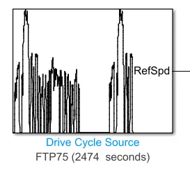
The Drive Cycle Source block generates a standard or user-specified longitudinal drive cycle. The block output is the specified vehicle longitudinal speed, which you can use to:
Predict the engine torque and fuel consumption that a vehicle requires to achieve desired speed and acceleration for a given gear shift reference. Produce realistic velocity and shift references for closed loop acceleration and braking commands for vehicle control and plant models. Study, tune, and optimize vehicle control, system performance, and system robustness over multiple drive cycles.
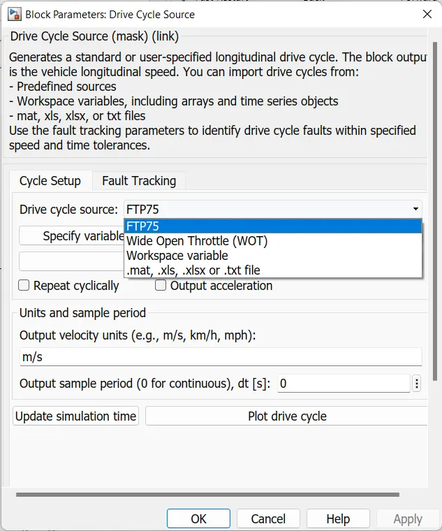
Drive cycles from predefined sources. By default, the block includes the FTP–75 drive cycle. To install additional drive cycles from a support package, see Install Drive Cycle Data. The support package has driven cycles that include the gear shift schedules, for example, JC08 and CUEDC.
Workspace variables that define your own drive cycles.
.mat, .xls, .xlsx, or .txt files.
Wide open throttle (WOT) parameters, including initial and nominal reference speed, deceleration start time, and final reference speed.
the above figure shows the drive cycle source properties. From the drive cycle source, we can choose the various types of drive cycles. And we can upload the drive cycle externally with different file formats (.mat, .xls, .xlsx, or .txt files.). This block is connected to the longitudinal driver block for the reference speed of the vehicle.
Longitudinal Driver:
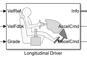
The Longitudinal Driver block implements a longitudinal speed-tracking controller. Based on reference and feedback velocities, the block generates normalized acceleration and braking commands that can vary from 0 through 1. You can use the block to model the dynamic response of a driver or to generate the commands necessary to track a longitudinal drive cycle.
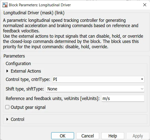
The longitudinal driver block has the input ports of velref, velFdbk, and Grade. Output ports Info, AccelCmd, and DecelCmd. The vehicle speed is taken as reference velocity feedback speed and the longitudinal driver block calculates and gives commands of acceleration and deceleration commands to the power converter block. This driver block has different typer os control types PI, Scheduled PI, and Predictive. Grade port is grounded because we are not taking the any grade input parameters.
MOTOR CONTROLLER:
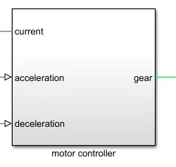
This motor controller subsystem consists of a DC motor, H-Bridge, controlled PWM voltage, controlled voltage source, current sensor, electrical reference, PS-Simulink converter, and mechanical reference blocks.
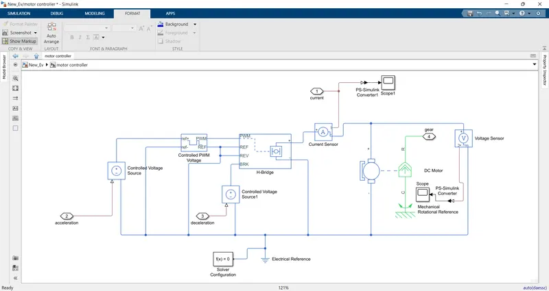
The above figure shows the motor control subsystem.
Controlled Voltage Source:

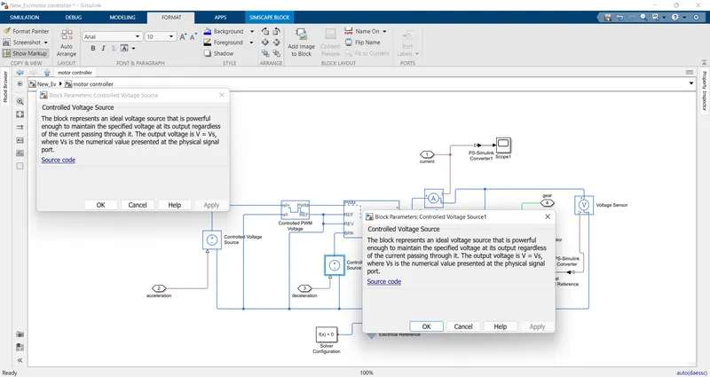
The Controlled Voltage Source block represents an ideal voltage source that is powerful enough to maintain the specified voltage at its output regardless of the current flowing through the source. The output voltage is V = Vs, where Vs is the numerical value presented at the physical signal port.
In this subsystem, we are using two controlled voltage source blocks. The first controlled voltage block positive terminal is connected to the controlled PWM voltage block positive terminal. The negative terminal is connected to PWM blocks negative reference input terminal and then the reference terminal is connected to the driver blocks acceleration terminal.
The second controlled voltage source blocks positive terminal is connected to H-Bridge BRK terminal, negative terminal is connected to common and electrical reference block and then the reference terminal is connected to breaking command terminal of longitudinal driver block.
The below figure shows the controlled voltage blocks.
Controlled PWM Voltage:
The Controlled PWM Voltage block represents a pulse-width modulated (PWM) voltage source. You can model electrical or physical signal input ports by setting the Modeling option parameter to either the block calculates the duty cycle based on the reference voltage across its ref+ and ref- ports. This option is the default. PS input Specify the duty cycle value directly by using an input physical signal port.
Block diagram of PWM voltage is shown below:

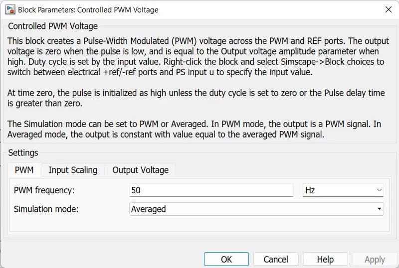
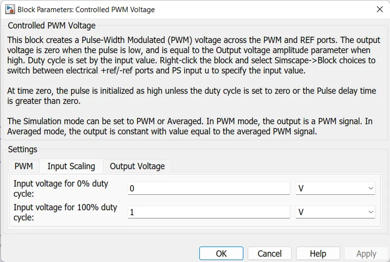
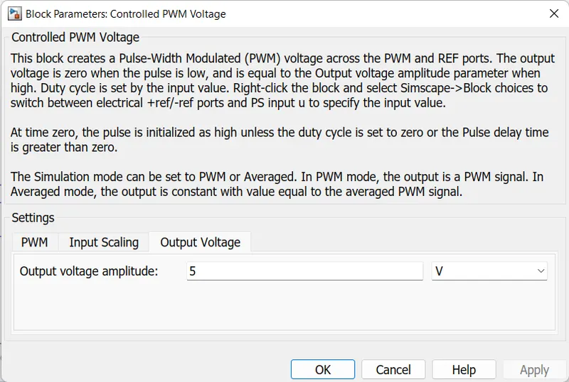
The controlled PWM Voltage positive reference port is connected to the positive terminal of the controlled voltage source, negative reference port is connected to the common ground terminal. The PWM port is connected to the H-Bridge PWM port, and then the REF port is connected to the common ground terminal. The Controlled PWM voltage block parameters are: PWM frequency is 50 Hz and simulation mode is Averaged. Input scaling parameters are Input voltage for 0% duty cycle is zero volts and then Input voltage for 100% duty cycle is 1v. The output voltage amplitude is 5V.
The PWM Block parameters are shown below:
H-Bridge:
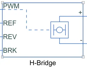
The H-Bridge block represents an H-bridge motor driver. The block has the following two Simulation mode options:
PWM — The H-Bridge block output is a controlled voltage that depends on the input signal at the PWM port. If the input signal has a value greater than the Enable threshold voltage parameter value, the H-Bridge block output is on and has a value equal to the value of the Output voltage amplitude parameter. If it has a value less than the Enable threshold voltage parameter value, the block maintains the load circuit using one of the following three Freewheeling mode options:
- Via one semiconductor switch and one freewheeling diode
- Via two freewheeling diodes
- Via two semiconductor switches and one freewheeling diode
The first and third options are sometimes referred to as a synchronous operation.
The signal at the REV port determines the polarity of the output. If the value of the signal at the REV port is less than the value of the Reverse threshold voltage parameter, the output has positive polarity; otherwise, it has negative polarity.
Averaged — This mode has two Load current characteristics options:
- Smoothed
- Unsmoothed or discontinuous
The Smoothed option assumes that the current is practically continuous due to load inductance. In this case, the H-Bridge block output is:
Vo.VPWM/APWM − IOUTRON
where:
- VO is the value of the Output voltage amplitude parameter.
- VPWM is the value of the voltage at the PWM port.
- APWM is the value of the PWM signal amplitude parameter.
- IOUT is the value of the output current.
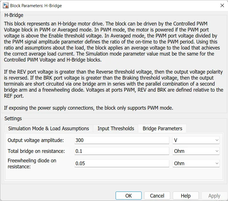
- RON is the Bridge on the resistance parameter.
The current will be smooth if the PWM frequency is large enough. Synchronous operation where freewheeling is via a bridge arm back to the supply also helps smooth the current. For cases where the current is not smooth, or possibly discontinuous (that is, it goes to zero between PWM cycles), use the Unsmoothed or discontinuous option. For this option, you must also provide values for the Total load series resistance, Total load series inductance, and PWM frequency. During simulation, the block uses these values to calculate a more accurate value for H-bridge output voltage that achieves the same average current as would be present if simulating in PWM mode.
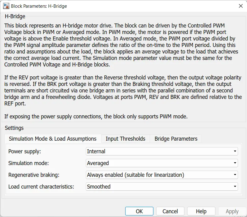
Set the Simulation mode parameter to Averaged to speed up simulations when driving the H-Bridge block with a Controlled PWM Voltage block. You must also set the Simulation mode parameter of the Controlled PWM Voltage block to Averaged mode. This applies the average of the demanded PWM voltage to the motor. The accuracy of the Averaged mode simulation results relies on the validity of your assumption about the load current. If you specify that the current is Unsmoothed or discontinuous, then the accuracy also depends on the values you provide for load resistance and inductance being representative. This mode also makes some simplifying assumptions about the underlying equations for the case when the current is discontinuous. For typical motor and bridge parameters, accuracy should be within a few percent. To verify Averaged mode accuracy, run the simulation using the PWM mode and compare the results to those obtained from using the Averaged mode.
Braking mode is invoked when the voltage presented at the BRK port is larger than the Braking threshold voltage. Regardless of whether in PWM or Averaged mode, when in braking mode the H-bridge is modeled by a series combination of two resistances R1 and R2 where:
- R1 is the resistance of a single bridge arm, that is, half the value of the Total bridge on the resistance parameter.
- R2 is the resistance of a single bridge arm in parallel with a diode resistance, that is, R1 · Rd / ( R1 + Rd ), where Rd is the diode resistance.
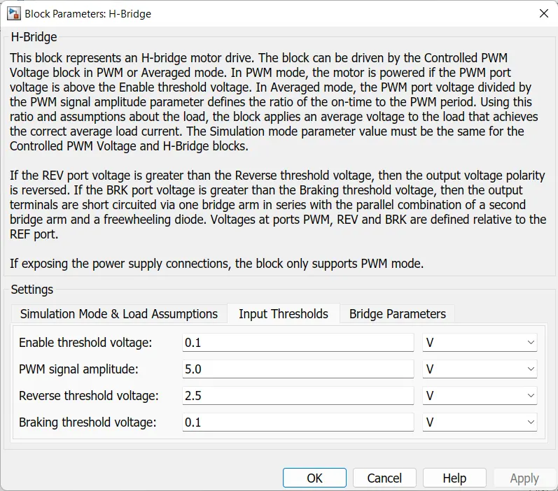
H-Bridge parameters:
CURRENT SENSOR:
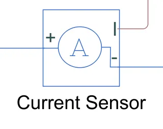
The block represents an ideal current sensor, that is, a device that converts current measured in any electrical branch into a physical signal proportional to the current.
Connections + and - are conserving electrical ports through which the sensor is inserted into the circuit. The connection I is a physical signal port that outputs current value.
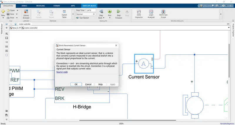
The current sensor positive input terminal is connected to the H-Bridge Positive terminal and the negative terminal of the current sensor is connected to the DC motor positive terminal. The reference port is connected to the controlled current source common terminal, and for analyzing the current parameters a scope is connected to the current sensor common terminal with a ps-Simulink converter block. This block converts the physical signal into a Simulink signal.
PS-Simulink Converter :

The PS-Simulink Converter block converts a physical signal into a Simulink® output signal. Use this block to connect outputs of a Simscape™ physical network to Simulink scopes or other Simulink blocks.

Simulink-PS Converter :

The Simulink-PS Converter block converts the input Simulink® signal into a physical signal. Use this block to connect Simulink sources or other Simulink blocks to the inputs of a Simscape™ physical network.

DC MOTOR:
This block represents the electrical and torque characteristics of a DC motor.
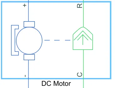
The block assumes that no electromagnetic energy is lost, and hence the back-emf and torque constants have the same numerical value when in SI units. Motor parameters can either be specified directly or derived from the no-load speed and stall torque. If no information is available on armature inductance, this parameter can be set to some small non-zero value.
When a positive current flows from the electrical + to - ports, a positive torque acts from the mechanical C to R ports. Motor torque direction can be changed by altering the sign of the back-emf or torque constants.
The DC motor positive terminal is connected to the current sensor negative terminal and voltage sensor positive terminal.
The negative terminal is connected to the common. the mechanical rotation terminal C is connected to the Mechanical Rotational reference block. then the R port is connected to the simple Gear.
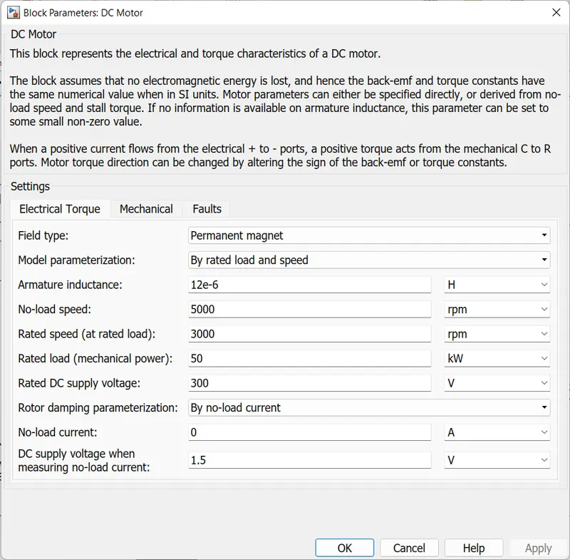
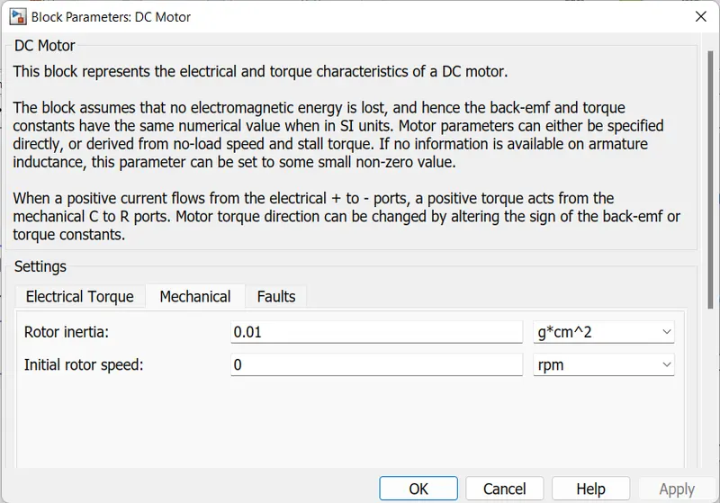
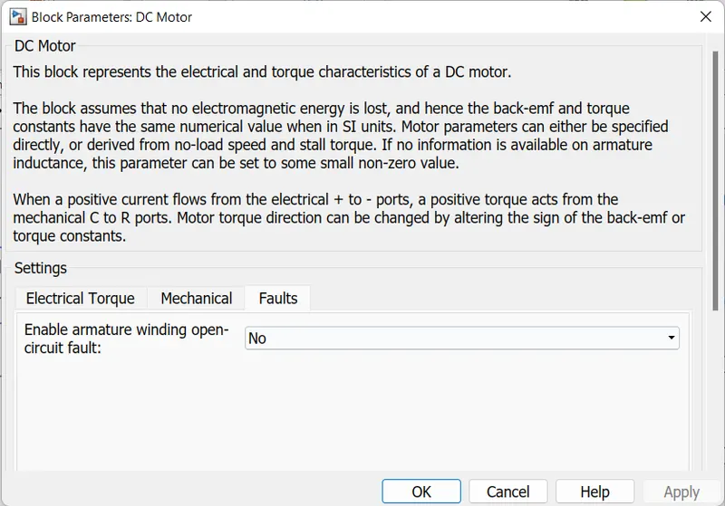
The following figures show the properties of the DC motor. here we are taking the rated load and speed values. we are taking no losses in this model.
Mechanical Rotational Reference:
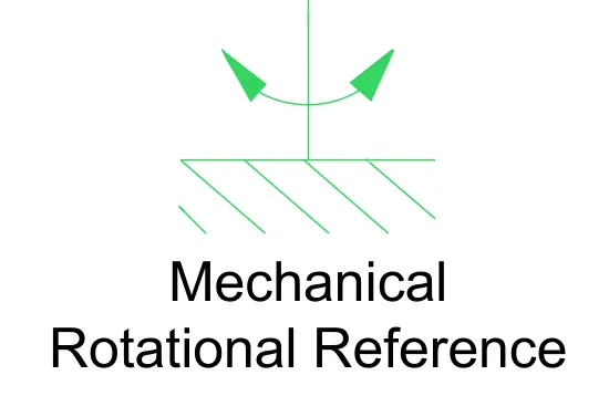
This block represents a mechanical rotational reference point, that is, a frame or a ground. Use it to connect mechanical rotational ports that are rigidly affixed to the frame (ground). this mechanical rotational reference block is connected to dc motor mechanical C port.
Voltage Sensor:
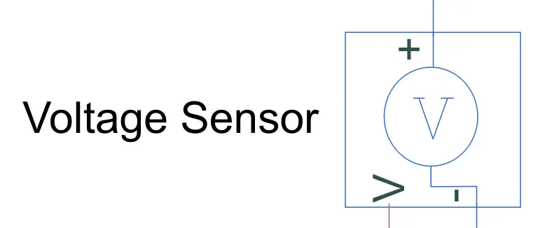
The Voltage Sensor block represents an ideal voltage sensor, that is, a device that converts voltage measured between two points of an electrical circuit into a physical signal proportional to the voltage.
Use the + and - ports to connect the sensor in parallel with the block (or several blocks) where you want to measure the voltage. Port V outputs the measurement result as a physical signal. Use a PS-Simulink Converter block to connect this port to Simulink® blocks, such as Scope or Display.
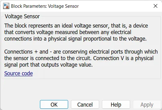
This voltage sensor block positive terminal is connected to the DC motor positive terminal, negative terminal of voltage sensor is connected to DC motor negative terminal, and then the common port is connected to scope through PS- Simulink converter block. This block converts the physical signal to the Simulink signal. Voltage sensor block properties are shown below.
Solver Configuration:
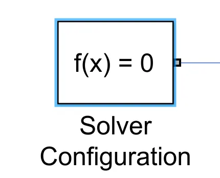
Each physical network represented by a connected Simscape™ block diagram requires solver settings information for simulation. The Solver Configuration block specifies the solver parameters that your model needs before you can begin the simulation. Each topologically distinct Simscape block diagram requires exactly one Solver Configuration block to be connected to it.
solver block is connected to the common ground block.
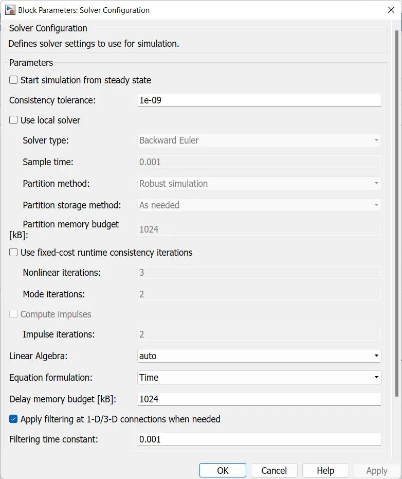
The block parameters of solver configuration are shown below:
Electrical Reference:
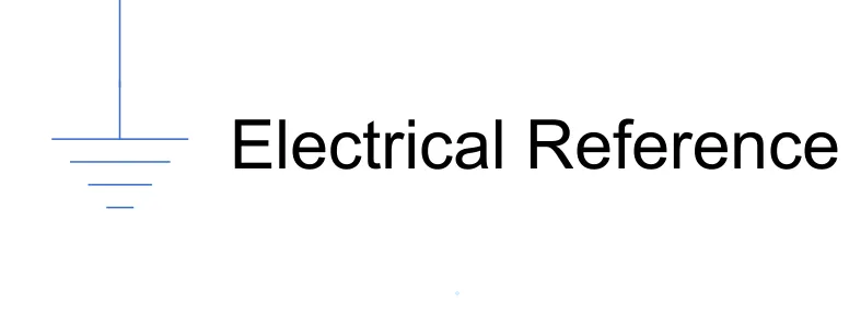
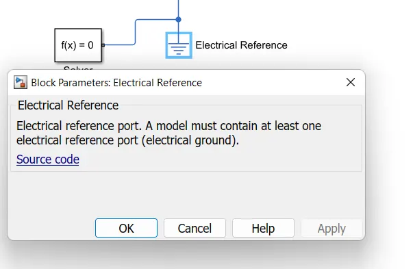
The Electrical Reference block represents an electrical ground. Electrical conserving ports of all the blocks that are directly connected to the ground must be connected to an Electrical Reference block. A model with electrical elements must contain at least one Electrical Reference block.
Connection Port:

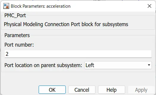
The Connection Port block transfers a physical connection or signal across subsystem boundaries. Physical connections include Simscape™ conserving and physical signal connections, Simscape Multibody connections, and Vehicle Dynamics Block set two-way connection ports, among others. This block is similar in function to the Inport and Outport blocks in the Simulink® library.
A subsystem needs a Connection Port block for each physical connection line that crosses its boundary. You can manually place a Connection Port block inside a subsystem, or Simulink can automatically insert a Connection Port block when you create a subsystem within an existing network.
The connection port block parameters figure is shown below:
Scope:
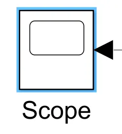
In the scope block, we can observe the plots. We can add more signal ports to view another plot in one scope block. We can select the legend option in the plot to view the name of the plot. We can change the line styles, colours and adjustment of the x, and y-axis.
Battery Subsystem:
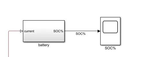
This battery subsystem is providing a supply to the dc motor to run. And in this subsystem, we can observe the battery SOC calculation blocks. This soc is tell us how much battery is used for the motor running. The below figure shows the battery subsystem.
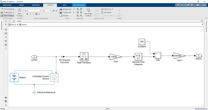
List of the block used in the battery subsystem:
- Battery block
- Controlled Current Source block
- PS-Simulink converter block
- Rate Transmission block
- Gain block
- Discrete-time integrator block
- Add block
- Constant block
- Connecting port block
- Out port block
Battery:
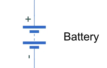
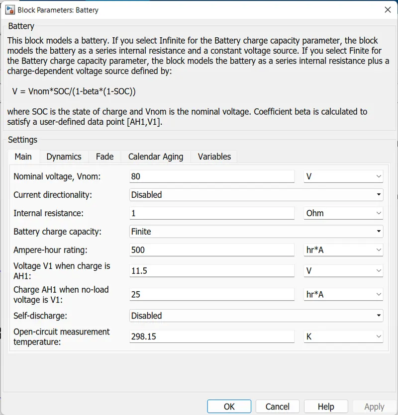
This block models a battery. If you select Infinite for the Battery charge capacity parameter, the block models the battery as a series of internal resistance and a constant voltage source. If you select Finite for the Battery charge capacity parameter, the block models the battery as a series of internal resistance plus a charge-dependent voltage source defined by:
V = Vnom*SOC/(1-beta*(1-SOC))
where SOC is the state of charge and Vnom is the nominal voltage. Coefficient beta is calculated to satisfy a user-defined data point [AH1, V1].
The battery-positive terminal is connected to the Rconn port, negative terminal of the battery is connected to the Lconn port of the controlled voltage source block. The below figure shows the battery parameters.
Controlled Current Source:
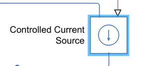
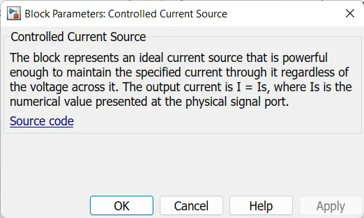
The block represents an ideal current source that is powerful enough to maintain the specified current through it regardless of the voltage across it. The output current is I = Is, where Is is the numerical value presented at the physical signal port.
This block is connected to the battery with Lconn and Rconn ports. Then its common port is connected to the connection port named as the current for the motor supply. Then it is also connected to the PS- Simulink converter block.
Rate Transition Block:
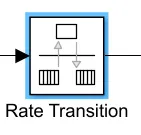
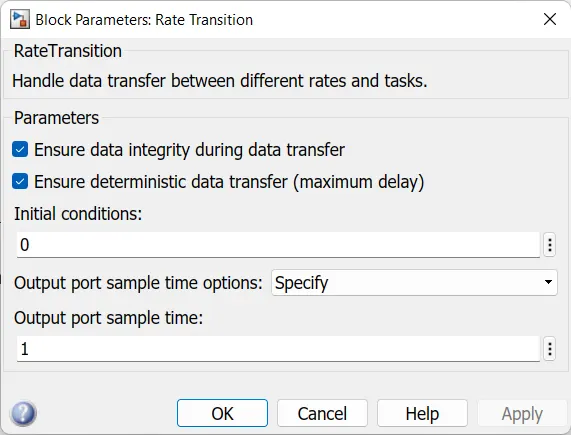
The Rate Transition block transfers data from the output of a block operating at one rate to the input of a block operating at a different rate. Use the block parameters to trade data integrity and deterministic transfer for faster response or lower memory requirements.
This block is having one input and one output terminal. The input port is connected to the PS Simulink converters output terminal and the output port is connected to the gain block. This rate transition block is transferring the data of battery current to SOC calculation.
Gain:

The Gain block multiplies the input by a constant value (gain). The input and the gain can each be a scalar, vector, or matrix.
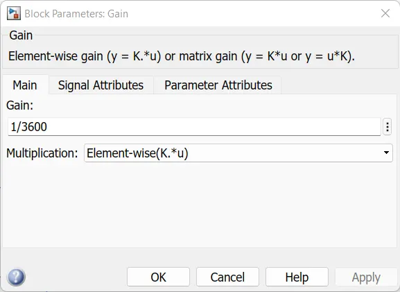
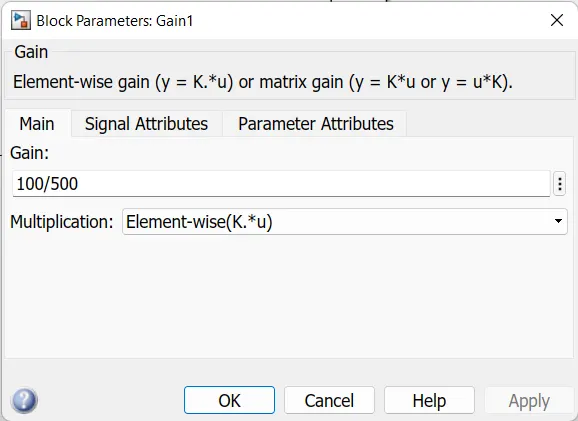
We can specify the value of gain in the Gain parameter. The Multiplication parameter lets you specify element-wise or matrix multiplication. For matrix multiplication, this parameter also lets you indicate the order of the multiplicands.
Gain is converted from doubles to the data type specified in the block mask offline using round-to-nearest and saturation. The input and gain are then multiplied, and the result is converted to the output data type using the specified rounding and overflow modes.
Element-wise gain (y = K.*u) or matrix gain (y = K*u or y = u*K).
The two gain blocks parameters are shown below:
Discrete-time integrator:

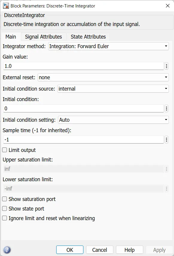
The Discrete-Time Integrator block is in place of the Integrator block to create a purely discrete model. With the Discrete-Time Integrator block, you can:
- Define initial conditions on the block dialog box or as input to the block
- Define an input gain (K) value
- Output the block state
- Define upper and lower limits on the integral
- Reset the state with an additional reset input
ADD Block:
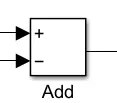
The addition block is used to add two or more inputs and give one output value. In this block, we can do the addition and multiplication operations by changing the signs of mathematical operations. In this model, we are adding the output of discrete time integrator and constant block values. The output of the addition block is given to the constant block.
Constant:

The Constant block generates a real or complex constant value signal. Use this block to provide a constant signal input. The block generates scalar, vector, or matrix output, depending on:
- The dimensionality of the Constant value parameter
- The setting of the Interpret vector parameters as 1-D parameter
The output of the block has the same dimensions and elements as the Constant value parameter. If you specify for this parameter a vector that you want the block to interpret as a vector, select the Interpret vector parameters as a 1-D check box. Otherwise, if you specify a vector for the Constant value parameter, the block treats that vector as a matrix.
The remaining blocks of this subsystem are Electrical Reference, connection port, and ps-Simulink blocks are discussed in the motor controller subsystem.
Transmission:
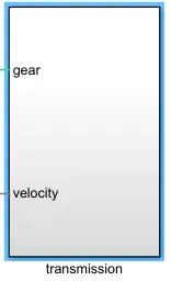
The transmission system contains vehicle wheels, gears, and vehicle body blocks. These are mechanical components that connected each other and drive the vehicle smoothly. This transmission subsystem is shown below.
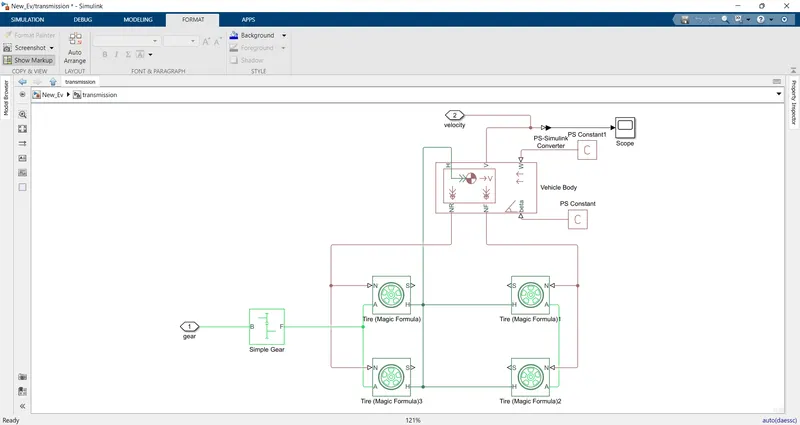
Blocks used in the transmission subsystem:
- Vehicle Body
- Tire (Magic Formula)
- Simple Gear
- PS to Simulink Converter
- PS constant
- Scope
- Connecting port
Vehicle Body:
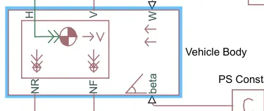
Represents a two-axle vehicle body in longitudinal motion. The block accounts for body mass, aerodynamic drag, road incline, and weight distribution between axles due to acceleration and road profile. The vehicle can have the same or a different number of wheels on each axle. Optionally include pitch and suspension dynamics or additional variable mass and inertia. The vehicle does not move vertically relative to the ground.
Connection H is the mechanical translational conserving port associated with the horizontal motion of the vehicle body. The resulting traction motion developed by tires should be connected to this port. Connections V, NF, and NR are physical signal output ports for vehicle velocity and front and rear normal wheel forces, respectively. Wheel forces are considered positive if acting downwards. Connections W and beta are physical signal input ports corresponding to headwind speed and road inclination angle, respectively. If the variable mass is modeled, the physical signal input ports CG and M are exposed. CG accepts a two-element vector representing the x and y distance offsets from vehicle CG to additional load mass CG. M represents the additional mass. If both variable mass and pitch dynamics are included, the physical signal port J accepts the inertia of the additional mass about its own CG.
The vehicle body is having the following ports:
NR- It is a rear axle force port.
NF- It is a front axle force port.
Beta – This is a road incline angle port.
H – This port is connected to the horizontal motion of the vehicle’s body.
V – it is a vehicle longitudinal velocity port.
W – is the Headwind speed port.
The vehicle body is a physical block, and the output signals are physical signals. The NR port is connected to the Rear wheels (left side) and the NF port is connected to the Front wheels (Right side). V port is connected to connecting port Velocity. Beta and W ports are connected to the PS Constant block.
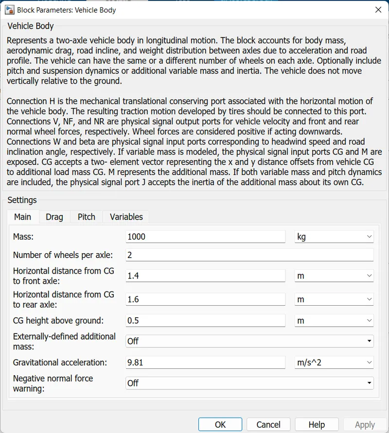
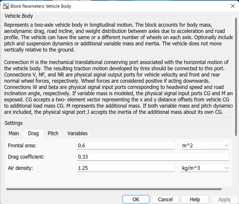
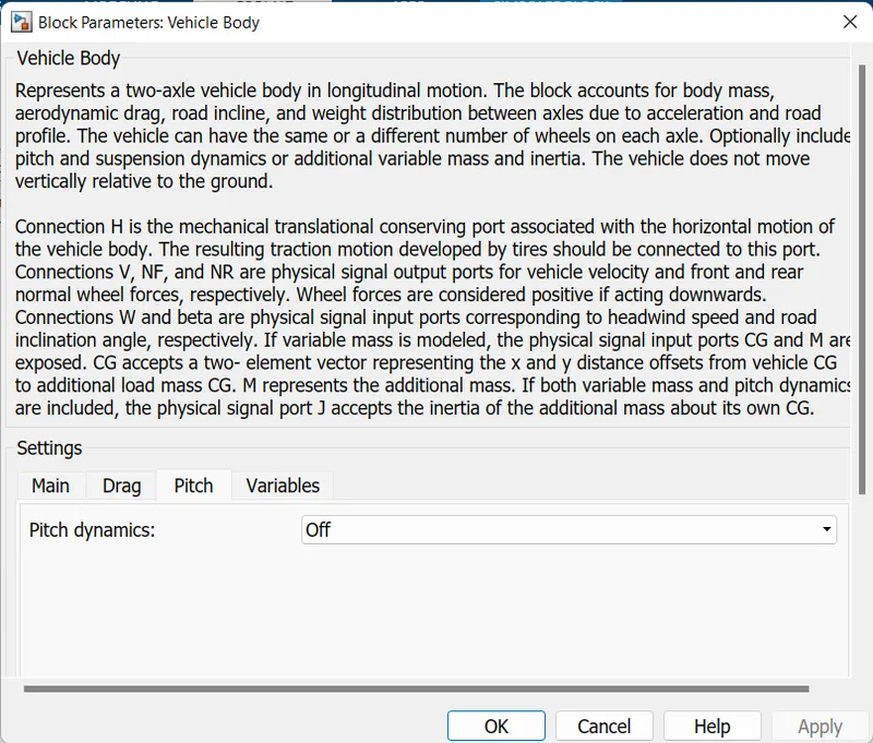
The vehicle body block parameters are shown below:
Tire (Magic Formula):
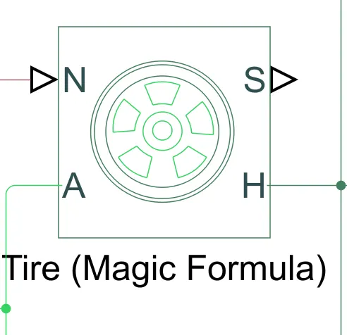
Represents the longitudinal behavior of a highway tire characterized by the tire Magic Formula. The block is built from Tire-Road Interaction (Magic Formula) and Simscape Foundation Library Wheel and Axle blocks. Optionally, the effects of tire inertia, stiffness, and damping can be included.
Connection A is the mechanical rotational conserving port for the wheel axle. Connection H is the mechanical translational conserving port for the wheel hub through which the thrust developed by the tire is applied to the vehicle. Connection N is a physical signal input port that applies the normal force acting on the tire. The force is considered positive if it acts downwards. Connection S is a physical signal output port that reports the tire slip. Optionally expose physical signal port M by setting Parameterize by to Physical signal Magic Formula coefficients. Physical signal port M accepts a four-element vector corresponding to the B, C, D, and E Magic Formula coefficients.
The tire block has the following ports:
N- This is a normal force connecting the port to the vehicle body.
A – This is the axle signal connecting the port.
S – this is a slip signal connecting the port.
H – this is a mechanical translational port. This wheel hub transmits the thrust generated by the tire.
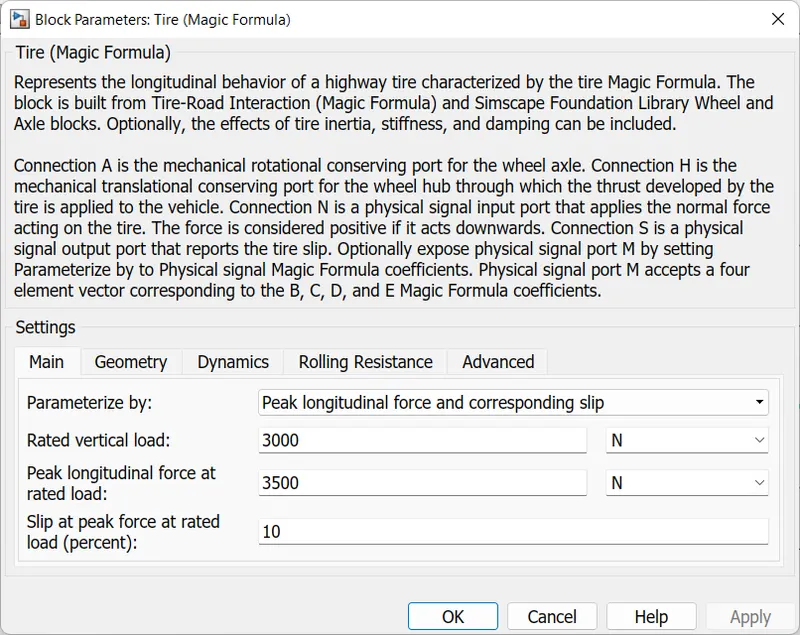
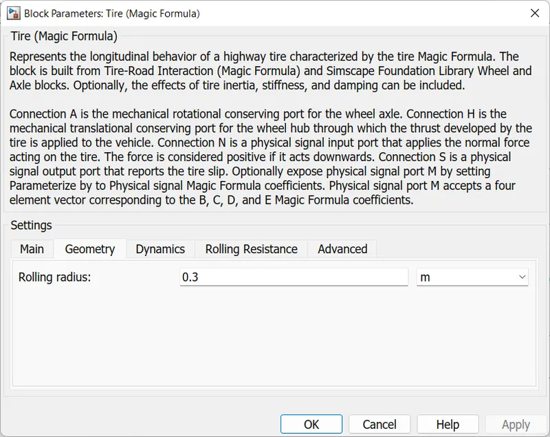
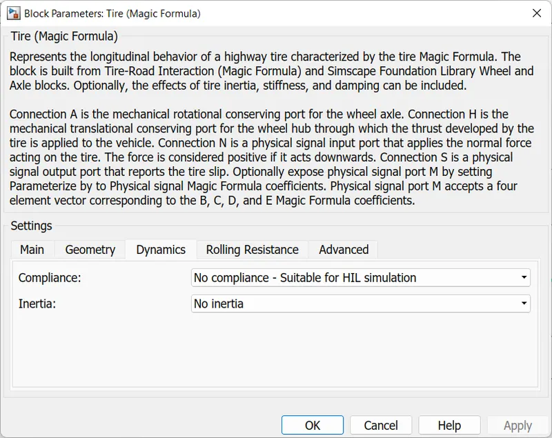
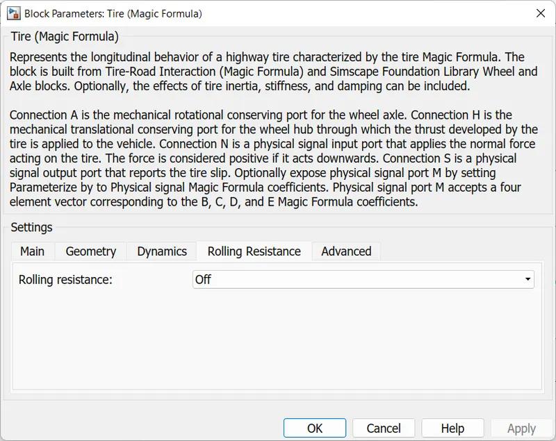
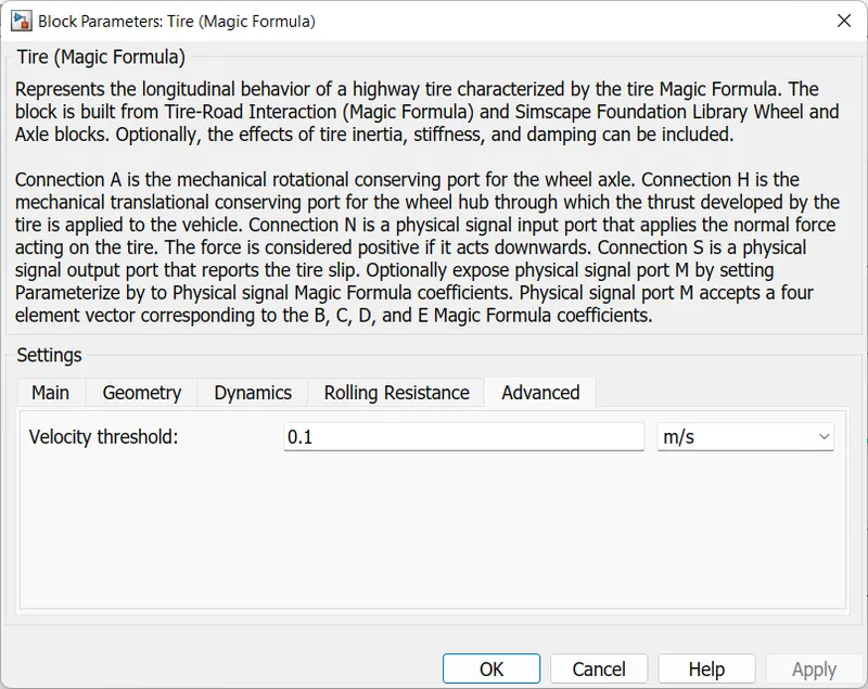
The left side tire’s (Rear Axle) N port is connected to the NR port of the vehicle body. The right side tire’s front wheels N port is connected to the NF terminal. H terminals are connected to the vehicle body H port. The S port is open, we are not taking any slip for the wheels. Tire block parameters are shown below figures:
PS Constant:
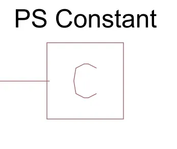
This block generates the physical signal of a constant value. The Constant parameter accepts both positive and negative values. The block output is a physical signal port. The PS constant block parameters are shown below.
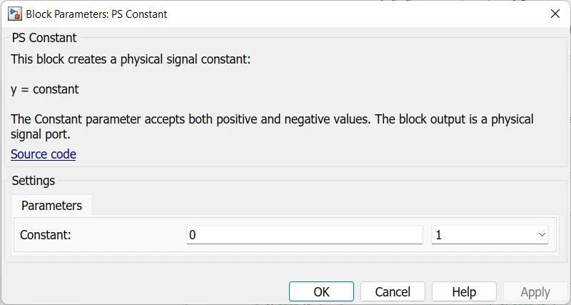
In this model, we are using two ps constant blocks for the beta angle and W ports. Beta and W port constants parameters are the same.
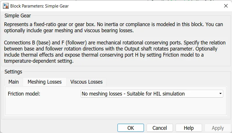
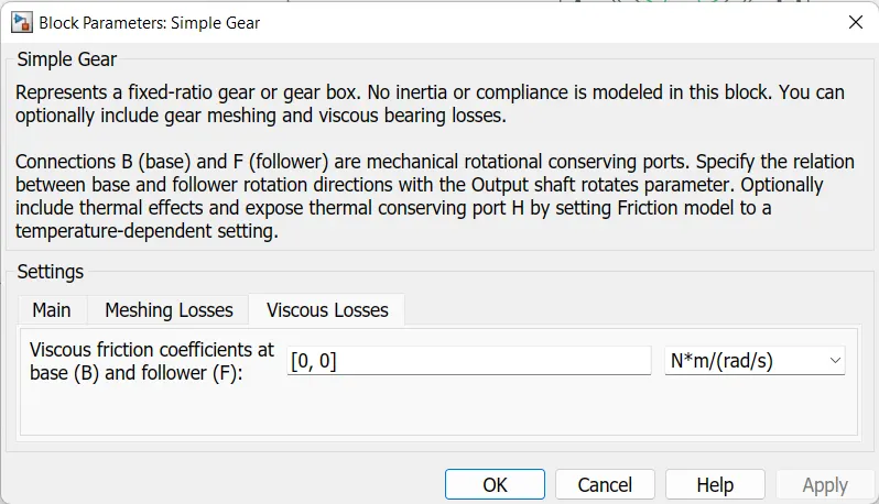
Simple Gear:
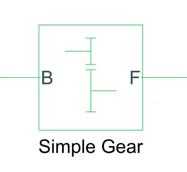
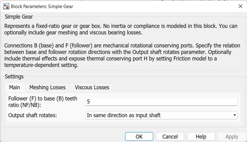
Represents a fixed-ratio gear or gearbox. No inertia or compliance is modeled in this block. You can optionally include gear meshing and viscous bearing losses.
Connections B (base) and F (follower) are mechanical rotational conserving ports. Specify the relation between base and follower rotation directions with the Output shaft rotates parameter. Optionally include thermal effects and expose thermal conserving port H by setting the Friction model to a temperature-dependent setting.
The simple gear block has one input port and one output port. The input port is connected to the motor controller gear output terminal. And the F port is connected to the real wheels Axle terminal.
The simple gear block parameters are shown below figures:
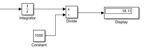
Here we are taking the integrator block at the velocity feedback port. When the velocity is integrated with respect to the time, the total distance is covered from the initial position to the final position of the vehicle. The integrated output of distance is multiplied and divided by the constant value of 1000 to get the distance in Kilometres. The total distance in kilometres is visible in the display block.
Vehicle Simulation:
Here we developed the model of an electric car with a battery and DC Motor and required individual blocks from powertrain blocks.
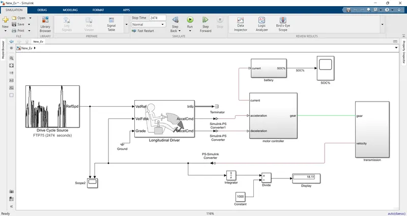
The simulation time is 2474seconds is taken as per the drive cycle run time. When the simulation is started the Drive Cycle Source is giving the reference speed as an input to the Longitudinal driver block and this block is having a controller. PI controller is used in the longitudinal driver block this was generating normalized acceleration and braking commands based on the reference and feedback velocities. The acceleration and deceleration commands are given to the motor controller block.
In the Motor Controller block, two controlled voltage source blocks are taken for acceleration and deceleration ports. When the Acceleration command is generated from the longitudinal driver block it is given to the controller voltage source common terminal. At time zero, the pulse is initialized as high unless the duty cycle is set to zero or the Pulse delay time is greater than zero. The output voltage is zero when the pulse is low and is equal to the Output voltage amplitude parameter when high. The duty cycle is set by the input value. This block represents an H-bridge motor drive. The block can be driven by the Controlled PWM Voltage block in PWM or Averaged mode. In PWM mode, the motor is powered if the PWM port voltage is above the Enable threshold voltage. In Averaged mode, the PWM port voltage divided by the PWM signal amplitude parameter defines the ratio of the on-time to the PWM period. Using this ratio and assumptions about the load, the block applies an average voltage to the load that achieves the correct average load current. The Simulation mode parameter value must be the same for the Controlled PWM Voltage and H-Bridge blocks. The PWM block positive output port is connected to the current sensor Positive input port. This current sensor converts the current measured in any electrical branch into a physical signal proportional to the current. The connection I is a physical signal port that outputs the current value. This output is given to the battery subsystems controlled current source common terminal. The motor positive terminal is connected to the current sensor negative terminal. Motor mechanical R port is connected to the simple gear. A voltage sensor is placed in parallel with DC Motor to measure the voltage. A solver is placed at common ground. In the transmission subsystem Gear is the input signal and the vehicle body is connected to the tires.
The vehicle body has the inclination angle and wind force ports these are connected to PS constant blocks. This vehicle body has an H port this port is connected to the wheel’s hub port of all four wheels. Tires force N port is connected to NR and NF these are rear force and font force. V port is the velocity of the vehicle body is output for the longitudinal driver block which is feedback.
In the battery subsystem, we are calculating the battery SOC. For this subsystem, the current is input, and output is connected to the scope to view the battery SOC. The battery is connected to the controlled current source common port is connected to the motor controller current sensor output port. The rate transition is transmitting the signal physical to Simulink form and it multiplied with gain then it was integrated with discrete time integrator and addition with some constant value it calculated with gain block.
To calculate the vehicle total distance covered by the vehicle, we took the feedback speed of the vehicle body and integrated it with an integrator. The output of the integrator speed is divided by 1000 to know the vehicle covered the distance in Kilometres.
Results:
When the developed model is simulated the below results, we can observe.
Scope 1:
The below-shown plot is observed for the scope which is connected to the Drive cycle source and Feedback velocity from the transmission subsystem.
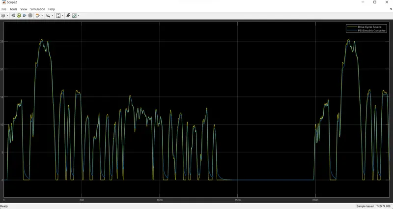
In this scope, we can observe the two plots which are the Drive cycle source and Feedback velocity. These plots are indicated in different colours yellow colour plot is the Drive cycle source and the blue one is feedback velocity. We can observe that both plots are similar with small variations. Sudden changes in acceleration and braking apply to the vehicle. Inclination angle and wind force acting on the vehicle also affect the vehicle performance. In real-time vehicle running vehicle drag force, acceleration, braking, and wind force are considered. These are affecting the vehicle speed as compared with reference drive cycle speed.
Scope-2:
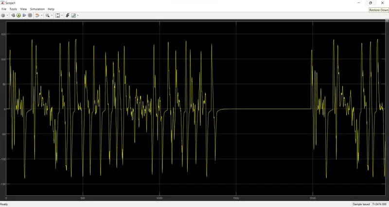
This plot is observed from the scope of the current sensor which is connected between the H-Bridge and DC motor.
The above plot observed the current variations of the motor according to the drive cycle. The current is increasing when the acceleration is applied and when the braking or deceleration command is applied current value is decreased. When the vehicle is at constant speed the current value also maintains constant. When the braking is applied the vehicle speed is decreasing and the current value is a negative region.
Scope-3:
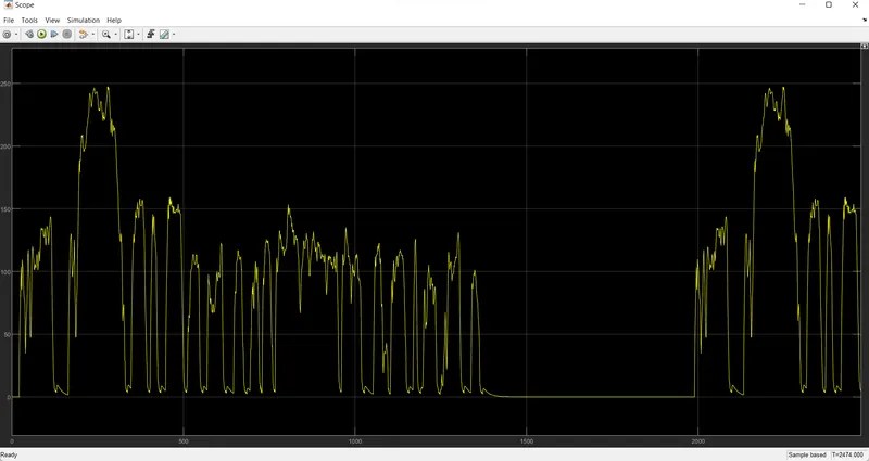
This plot is observed for the voltage variation across the DC motor. The voltage sensor is connected across the DC motor. The voltage is compared with the feedback velocity, we can observe the change in voltage respective to the velocity variations. When the vehicle is accelerated, voltage is also increasing and then the voltage is decreasing when the breaking is applied. The voltage is constant with the respective vehicle speed is constant.
Scope-4:
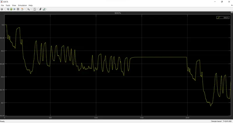
This plot is observed from the battery subsystem for the battery state of charge, charging, and discharging. When we compare this battery plot with the drive cycle plot we can observe, that when the vehicle is accelerating to high speed the battery consumption is high as a result the battery discharges more. When the braking is applied the vehicle is in regenerative braking mode so in this condition battery was getting charged, this variation we can view in the plot. We can see the battery discharging and charging in this scope.
Conclusion:
The MATLAB model of an electric car is created by using the Battery and DC motor. This model is Simulated and the vehicle Drive cycle, Feedback velocity, Current, Voltage, and %SOC are observed through the scopes. The difference in parameters performance is analyzed and discussed step by step with the plots. Each block’s operation and connections are explained clearly with their images. The vehicle system level configurations are explained with pictorial representation. The results are analyzed and explained clearly with their plots.