Final Project: Design of an Electric Vehicle

PROJECT: DESIGN OF AN ELECTRIC VEHICLE

AIM: -

Creating a MATLAB model of an Electric car that uses a battery and a DC motor. Prepare a report about the model including the following objectives

1. System Level configurations
2. Model parameters
3. Results
4. Conclusion

DESCRIPTION: -

ELECTRIC VEHICLE:

An electric vehicle (EV) is a vehicle that uses one or more electric motors for propulsion. It can be powered by a collector system, with electricity from extravehicular sources, or it can be powered autonomously by a battery. EVs include, but are not limited to, road and rail vehicles, surface and underwater vessels, electric aircraft, and electric spacecraft.

ELECTRIC CAR:

An electric car (battery-electric car, or all-electric car) is an automobile that is propelled by one or more electric motors, using only energy stored in batteries. Compared to internal combustion engine (ICE) vehicles, electric cars are quieter, have no exhaust emissions, and have lower emissions overall.

Components of Electric Car:

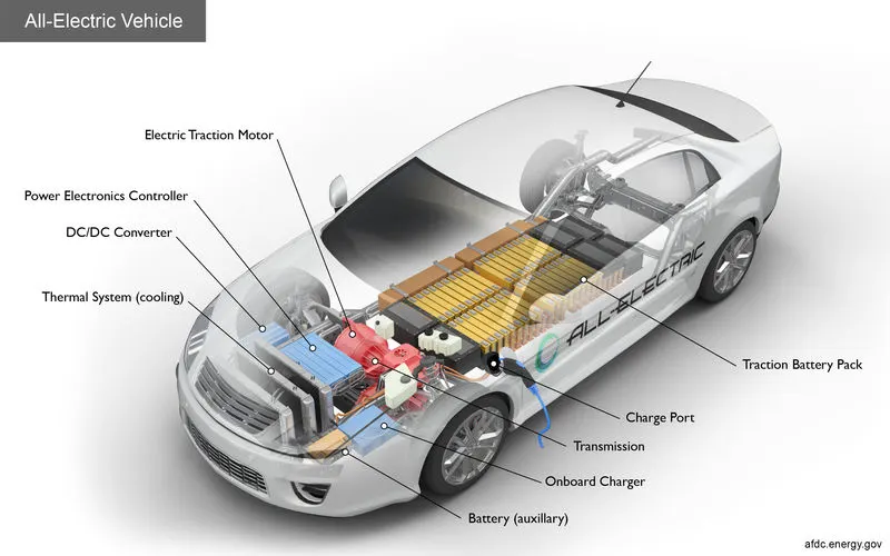
The major components making the car efficient are listed and briefed below.

• Battery (All-Electric Auxiliary)
• Charge Port
• DC / DC Converter
• Electric Traction Motor
• On-board Charger
• Power Electronics Controller
• Thermal System (Cooling)
• Traction Battery Pack
• Transmission (Electric)

1. Battery (All-Electric Auxiliary): A Battery is an electrochemical system that converts chemical energy into electrical energy. Battery-Cells are the most basic individual component of a battery. The auxiliary battery furnishes electricity to power vehicle accessories in an Electric vehicle.
2. Traction Battery Pack: An EV traction battery is rechargeable energy storage that supplies power to the electric motor very quickly, giving EVs high performance & rapid acceleration.
3. Charge Port: To power the traction battery pack, the vehicle has to connect to the external power supply which the charge port allows.
4. Onboard Charger: Monitoring battery traits, such as the current, temperature, voltage, and the state of charge while charging the pack. The process is of input of AC electricity supplied via the charge port converting it to DC power for the traction battery charging.
5. DC / DC Converter: For a smooth running of the vehicle accessories and recharge of the auxiliary batteries, the converter helps in converting the high voltage DC power from the traction battery pack to a lower voltage DC.
6. Power Electronics Controller: Controlling the speed of the electric traction motor with the torque it produces, the unit manages electrical energy flow which is delivered by the traction battery.
7. Electric Traction Motor: Power is taken from the traction battery pack and with this the motor drives the wheels of the vehicle. Some vehicles use motors that serve as drive as well as regeneration.
8. Transmission (Electric): Transfer of the mechanical power from the Electric Traction Motor which helps in driving the wheels.
9. Thermal System (Cooling): Thermal cooling helps in supporting a stable operating temperature range of the Electric Motor, Power Electronics Controller, and other components.

WORKING OF ELECTRIC CAR:

Electric Cars look the same as any regular fuel-generated Cars, however, Plug-in Cars don’t have the Tail Pipe and Gas Tank. The source of the power of the Electric Car is the batteries which act as Gas tanks, supplying the Electric Motor with the energy to run the vehicle. The battery’s Electrical energy gets converted into Kinetic energy by the Motor of an Electric Car.

The user/driver turns on the car or powers the car. Selects the “Forward” or “Reverse” option and step on the accelerator pedal. The electric motor has only a single rotating element called the Potentiometer. The motion from the motor is transmitted to the car wheels through the Controller. The power is controlled by the Controller which helps determine which parts or accessories require more power and thereby helps in the distribution of the battery energy.

If the Car has to move “Reverse” then the flow of electricity through the motor is reversed which changes the rotation of the Motor. This makes the wheels rotate in the opposite direction. The Electric Cars have a Regenerative braking system along with conventional friction braking.

In Regenerative Braking System, when the User/Driver releases the accelerator pedal and pushes the brakes, the motor acts as a generator and converts Car’s kinetic energy to electrical energy which helps in recharging batteries. This process reduces the speed of the Car. The User can also apply the conventional Friction braking system for stopping the car immediately. The rest of the components like the Air Bags and Air Conditioning are the same as the fuel-powered cars.

BLOCK DIAGRAM FOR MODELLING THE ELECTRIC CAR:

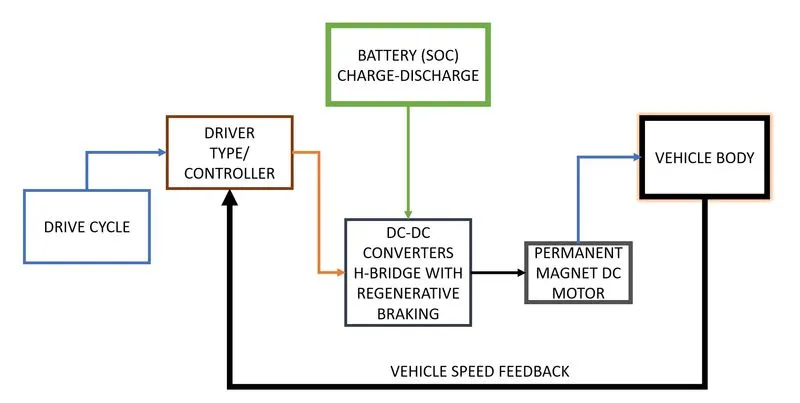
BLOCK DIAGRAM OF THE ELECTRIC CAR

EXPLANATION:

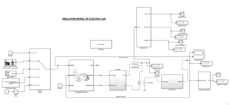
Block diagram of EV Car for modeling consists of the following blocks as mentioned below

1. Drive Cycle
2. Driver Type/Controller
3. DC-DC converters
4. DC Motor
5. Vehicle Body

A Drive cycle is a velocity-time profile that describes the driving characteristics of a specific type of vehicle under real-world driving conditions which will provide the commands to the Driver controller such as acceleration, deceleration, and braking signals will receive by the battery-connected DC-DC converter (H-Bridge with regenerative braking).

The signals are between 0 to 1 and those are the duty ratio command to the converter to provide the power supply from the battery to the permanent magnet DC motor.

The motor is connected to the vehicle body through the gear and the differential transmission is connected to the wheels. As per the command of the driver, the vehicle speed will accelerate and decelerate, and the same given feedback to the driver controller.

Approach to Modelling the EV Car:

The method of modeling the EV car will follow the below-mentioned approach

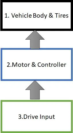
MODELLING OF EV CAR:

Vehicle Body and Tires-

1. Vehicle Body

The Vehicle body means that the entire chases of the vehicle consist of 6 ports which were Normal Reaction of Front and Rear (NR, NF), the Beta indicates the inclination of the road like gradeability, H represents the Hub, W represents the wind acting on the vehicle, V is the output velocity of the vehicle.

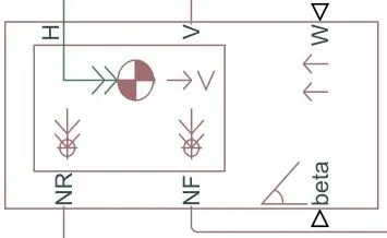
Configured parameters of the vehicle body as shown in the below picture

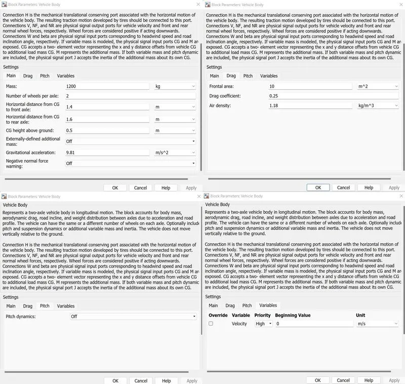
We have kept all the parameters as default except the frontal area we have taken as 10 m² and consider the rolling resistance with the default parameters.

2. Tires

The Tire (Magic Formula) block models a tire with longitudinal behavior given by the Magic Formula, an empirical equation based on four fitting coefficients. The block can model tire dynamics under constant or variable pavement conditions. The longitudinal direction of the tire is the same as its direction of motion as it rolls on the pavement. This block is a structural component based on the Tire-Road Interaction (Magic Formula) block. To increase the fidelity of the tire model, you can specify properties such as tire compliance, inertia, and rolling resistance. However, these properties increase the complexity of the tire model and can slow down the simulation. Consider ignoring tire compliance and inertia if simulating the model in real-time or if preparing the model for hardware-in-the-loop (HIL) simulation.

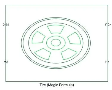
Configured parameters of the Tire as shown in the below picture, the same was applied to all four tires

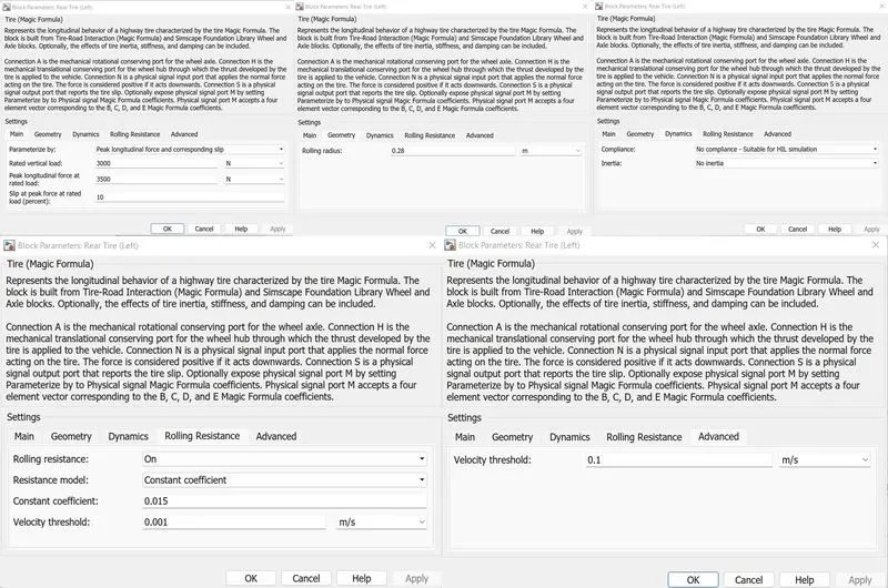
In the tire parameters, we have changed the tire radius to 0.28m respective to the frontal area of the vehicle body.

3. Simple Gear

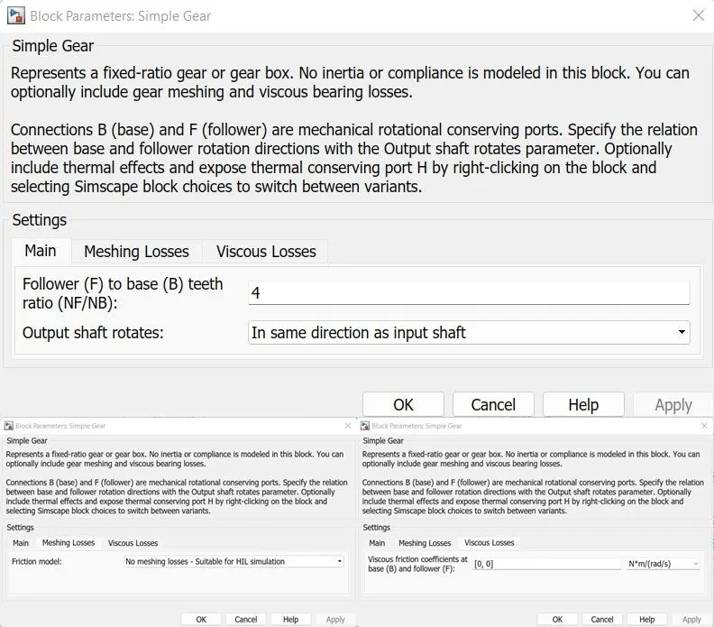
The Simple Gear block represents a gearbox that constrains the connected driveline axes of the base gear, B, and the follower gear, F, to corotate with a fixed ratio that you specify. You choose whether the follower axis rotates in the same or opposite direction as the base axis. If they rotate in the same direction, the angular velocity of the follower, ωF, and the angular velocity of the base, ωB, have the same sign. If they rotate in opposite directions, ωF and ωB have opposite signs.

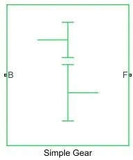
The output shaft is kept in the same direction to avoid the negative velocity, the block parameters of the were shown below.

4. Differential

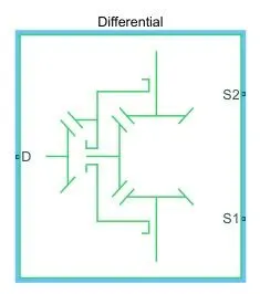
This block represents a gear mechanism that allows the driven shafts to spin at different speeds. Differentials are common in automobiles, where they enable the various wheels to spin at different speeds while cornering. Ports D, S1, and S2 represent the driving and driven shafts of the differential. Any of the shafts can drive the remaining two.

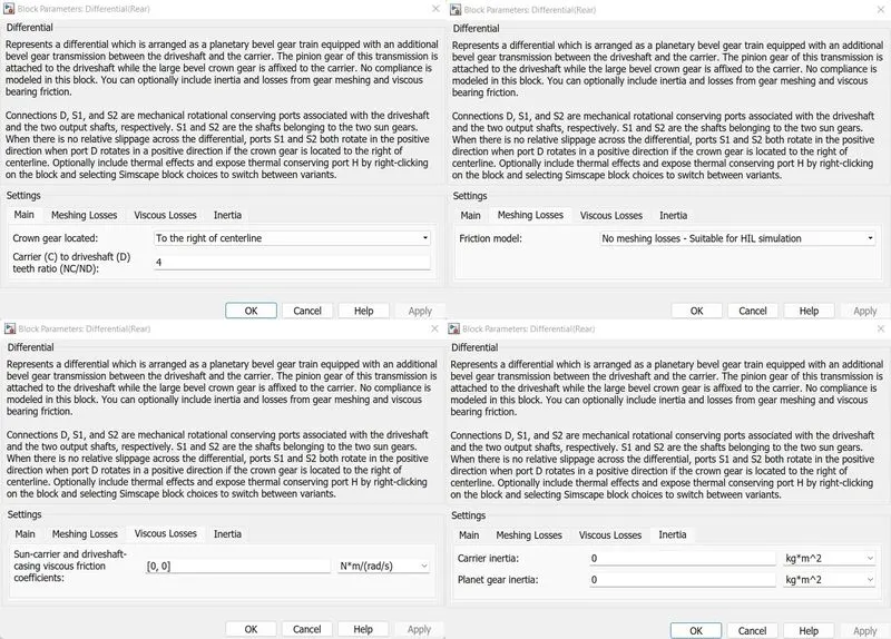
The block parameters of the differential block shown below same were applied for both blocks (Front, and rear) shown below.

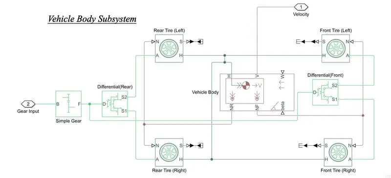
To model the Vehicle body subsystem, we have taken the 1 vehicle body block, 4 tire blocks, 2 differential blocks, and 1 simple gear. Positioned the 4 tires as, 2tires for the front and 2 tires for the rear.

Rear tires N port connected to the NR port of the vehicle body and Front tires N port connected to the NF port of the vehicle body.

Axle port A of the front tires is connected to S1 & S2 of the Differential front and Axle port A of the rear tires is connected to S1 & S2 of the Differential Rear. Both the D port of differential blocks are connected to the F port of Simple gear.

Hub port of the right-side tires got connected and same on the left-side tires, then both the Hub bus connected to the Hub port of vehicle body.

Slip port of all tires connected to terminator block to avoid the complexity in modeling. Since Tire was a physical system so by using the PS-Simulink converter block we connected the Slip to the Terminator block.

B port of the Simple gear will be the Input of the Vehicle body subsystem which will connect to the Motor and the V port of the vehicle body will be the output port of the subsystem.

The Vehicle body subsystem with the above-mentioned connections is shown below.

Motor and Controller-

1. DC Motor

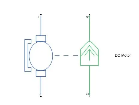
This is the DC Motor that would give the rotational power to the wheels and become the sole power generation source. The DC Motors terminals are connected as mentioned below,

+Ve = Electrical signal to the motor Positive Terminal

-Ve = Electrical signal to the motor Negative Terminal

R = Casing of the Motor connected with the Mechanical Rotational Reference Block

C = Rotor Case connected to the Simple gear.

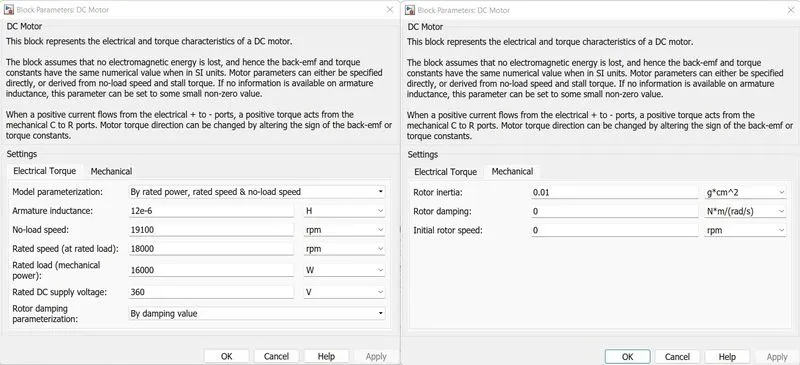
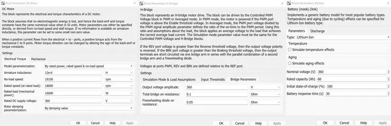
The model parameterization is considered as (By rated power, rated speed & no-load speed) The Armature inductance is as default, varied the changes in the No-Load Speed as 19100 rpm, the rated speed as 18000 rpm, the Rated Load at 16kW, and the Rated DC Supply Voltage as 360 V. All other parameters are as default.

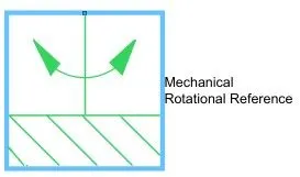
Mechanical Rotational Reference

The Mechanical Rotational Reference block represents a reference point, or frame, for all mechanical rotational ports. All rotational ports that are rigidly clamped to the frame (ground) must be connected to a Mechanical Rotational Reference block.

2. H-Bridge Converter with Regenerative Braking

H- bridge block output is a controlled voltage that depends on the input signal at the PWM port. The H- bridge is connected to Pulse Width Modulation for controlling the voltage signals and the output of the H bridge is connected to the terminals to provide the controlled voltage to the D.C motor.

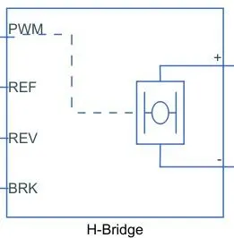
The ports in H- BRIDGE are:

Input Ports:

PWM – this stand for pulse width modulation which provides the voltage pulses to H- bridge either in PWM or average mode.

REF – is the floating zero-volt reference.

REV - Voltage that controls when to reverse the polarity of the H- bridge block output.

BRK – Voltage that controls when to short circuit the H-bridge block output.

Output Port:

+Ve = Electrical signal to the motor Positive Terminal

-Ve = Electrical signal to the motor Negative Terminal

Parameters Consideration:

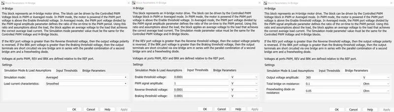
1. Averaged Simulation Mode and Smoothed load current characteristics so that the run-time of simulation will be faster.
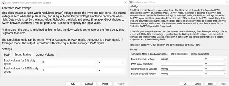
2. Kept all the threshold voltage values as lower = 0.0001 V and the PWM signal as 1V.
3. Amplitude of output voltage =360V, remaining bridge parameters kept same.

3. Controlled PWM Voltage

The Controlled PWM Voltage block represents a pulse-width modulated (PWM) voltage source that provides voltage to the H-bridge block.

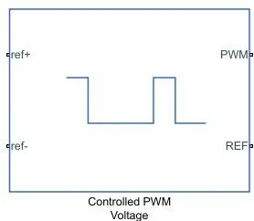
Ports ref+, ref- will get signals from the driver block such as acceleration and deceleration commands. PWM and REF are connected to the H-bridge and will provide the generated PWM signal to H-bridge.

Parameters Consideration:

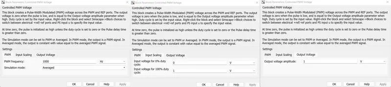
1. Averaged Simulation Mode considered and PWM frequency kept default.
2. Kept the duty cycle input voltage at 0% as 0V and at 100% as 1V.
3. Output voltage amplitude as 1V.

The overall H-bridge subsystem is shown below.

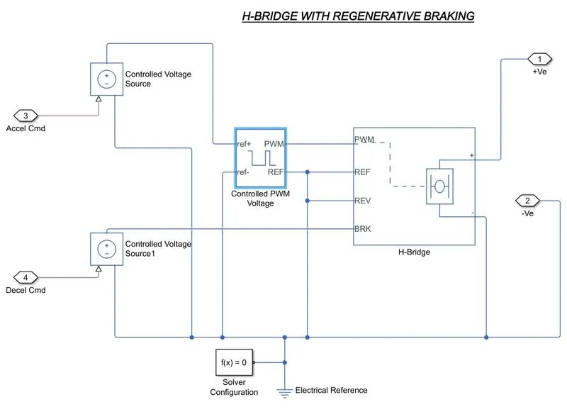
Controlled Voltage Source: The Controlled Voltage Source block represents an ideal voltage source that is powerful enough to maintain the specified voltage at its output regardless of the current flowing through the source. The block has one physical signal input port and two electrical conserving ports associated with its electrical terminals.

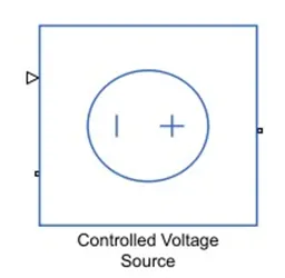
We have used this block that will receive the signal from the driver and the same will provide to PWM and H-Bridge

Current Sensor: The Current Sensor block represents an ideal current sensor, that is, a device that converts current measured in any electrical branch into a physical signal proportional to the current.

Connections + and – are electrical conserving ports through which the sensor is inserted into the circuit. The connection ‘I’ is a physical signal port that outputs the measurement result.

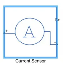
This block is used to measure the current flow to the motor which can be visualized from Scope and display blocks.

Electrical Reference

The Electrical Reference block represents an electrical ground. Electrical conserving ports of all the blocks that are directly connected to the ground must be connected to an Electrical Reference block. A model with electrical elements must contain at least one Electrical Reference block.

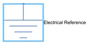
The Negative and -ref ports of the DC Motor, H-Bridge, PWM, controlled voltage source connected to the Electrical Reference.

Solver Configuration

Each physical network represented by a connected Simscape block diagram requires solver settings information for simulation. The Solver Configuration block specifies the solver parameters that your model needs before you can begin the simulation.

Each topologically distinct Simscape block diagram requires exactly one Solver Configuration block to be connected to it.

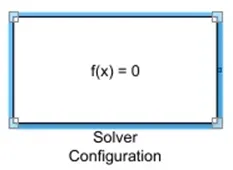
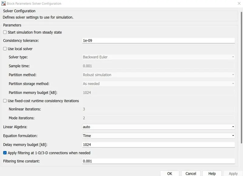
Connected the Solver configuration to the Electrical Reference.

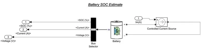
4. Battery SOC Estimate

The battery is connected as the power source to the model so that the power could be generated and the same power is transmitted accordingly to all the operating sources. The subsystem is to estimate Battery SOC after running the simulation.

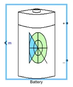
Battery

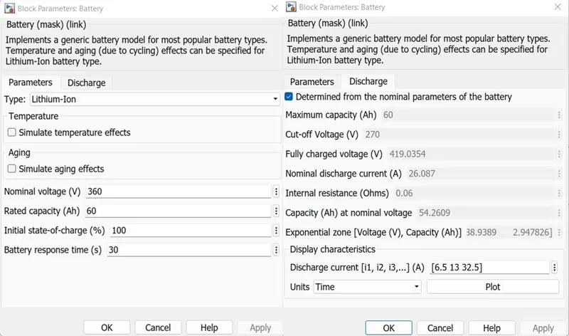
The Battery block implements a generic dynamic model parameterized to represent the most popular types of rechargeable batteries.

Taken the Battery type as Lithium-Ion with a rated voltage of 360V, 60AH capacity, and 100% of SOC.

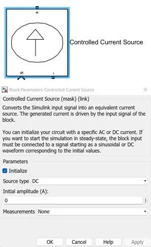
Controlled Current Source

This Controlled current source Converts the Simulink input signal into an equivalent current source. The generated current is driven by the input signal of the block. Block is connected in series to the Battery and chosen the source type as DC. It will receive the Motor current signal from the current sensor of the DC motor.

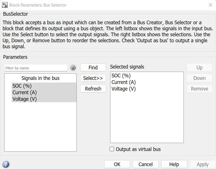
The m-port of the battery is connected to the Bus selector which will provide the output of the selected parameters. Here taken 3 output port bus selectors that provide the outputs of the Battery voltage, current, and SOC.

All the parameters can be visualized through Scope and Display.

NOTE:

In modeling the Motor and its controller below mentioned parameters need to be followed

• The rated DC voltage of the DC motor, Output voltage amplitude of H-Bridge, and Nominal voltage of the battery should be the same as shown below.

• The input voltage of PWM and the PWM signal amplitude of the H-Bridge should be 1V.

DRIVE INPUT: -

1. Longitudinal Driver-

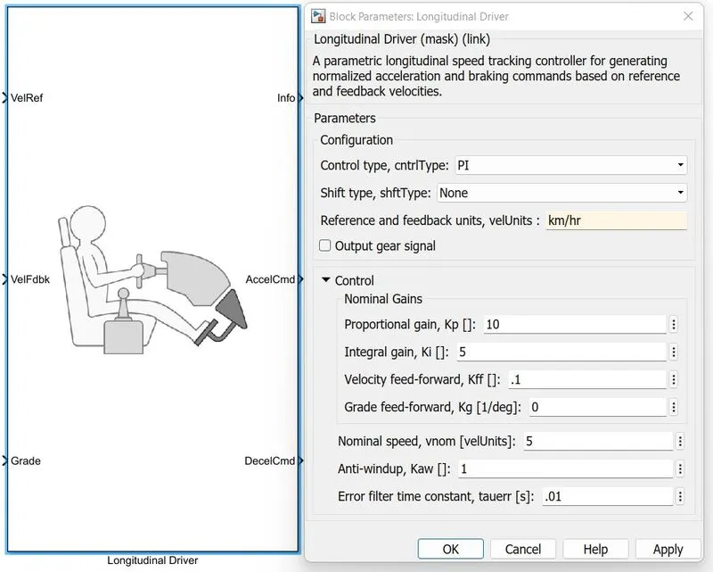
The Longitudinal Driver block implements a longitudinal speed-tracking controller. Based on reference and feedback velocities, the block generates normalized acceleration and braking commands that can vary from 0 through 1. We can use the block to model the dynamic response of a driver or to generate the commands necessary to track a longitudinal drive cycle. Here we have changed the units to km/hr.

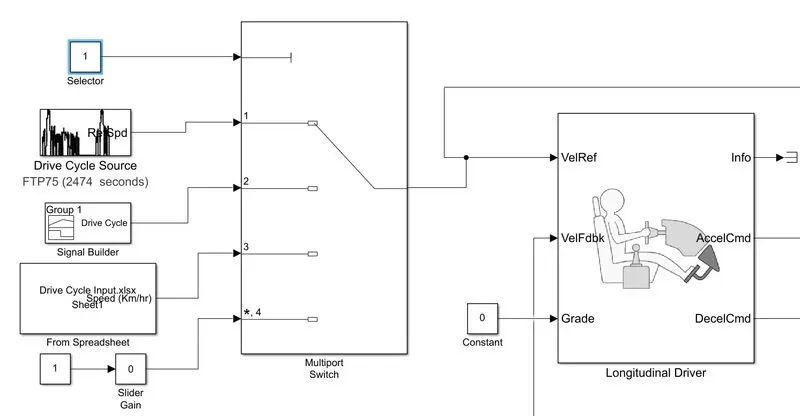
2. Multiport Switch-

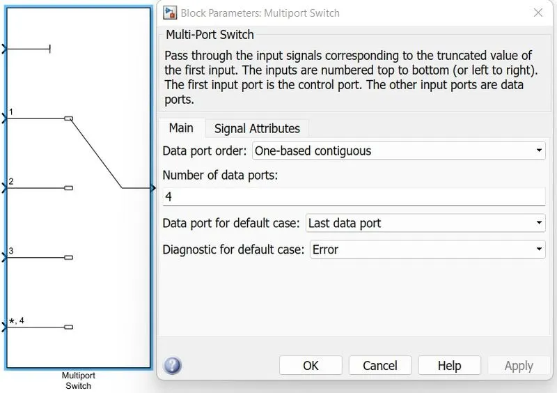
The Multiport Switch block determines which of several inputs to the block passes to the output. The block bases this decision on the value of the first input. The first input is the control input and the remaining inputs are the data inputs. The value of the control input determines which data input passes to the output.

3. Driving cycle Input-

We are providing the 4 types of driving cycle inputs mentioned below

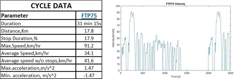
1. Drive Cycle Source (FTP75)
2. Signal Builder
3. From Spreadsheet (Time, km/hr)
4. Slider Gain.
5. Drive Cycle Source (FTP75)

The Drive Cycle Source block generates a standard or user-specified longitudinal drive cycle. The block output is the specified vehicle longitudinal speed, which you can use to:

• Predict the engine torque and fuel consumption that a vehicle requires to achieve desired speed and acceleration for a given gear shift reference.
• Produce realistic velocity and shift references for closed-loop acceleration and braking commands for vehicle control and plant models.
• Study, tune, and optimize vehicle control, system performance, and system robustness over multiple drive cycles.

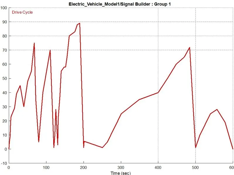
2. Signal Builder

The Signal Builder block allows you to create interchangeable groups of piecewise linear signal sources and use them in a model. You can quickly switch the signal groups into and out of a model to facilitate testing. In the Signal Builder window, create signals and define the output waveforms.

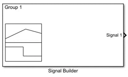
The created drive cycle input for this model with the time period of 600 secs shown below

3. From Spreadsheet (Time, km/hr)

The From Spreadsheet block reads data from Microsoft Excel (all platforms) or CSV (Microsoft Windows platform with Microsoft Office installed only) spreadsheets and outputs the data as a signal. The From Spreadsheet block does not support Microsoft Excel spreadsheet charts.

The From Spreadsheet icon displays the spreadsheet file name and sheet name specified in the block File name and Sheet name parameters.

3. From Spreadsheet (Time, km/hr)

The From Spreadsheet block reads data from Microsoft Excel (all platforms) or CSV (Microsoft Windows platform with Microsoft Office installed only) spreadsheets and outputs the data as a signal. The From Spreadsheet block does not support Microsoft Excel spreadsheet charts.

The From Spreadsheet icon displays the spreadsheet file name and sheet name specified in the block File name and Sheet name parameters.

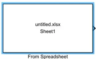
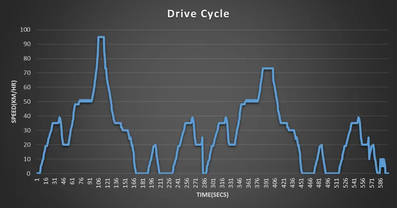
Prepared the drive cycle data to consist of time in secs for 600 sec and speed in km/hr, the plot of the prepared data is shown below.

4. Slider Gain.

The Slider Gain block performs a scalar gain that you can modify during simulation. Modify the gain using the slider parameter.

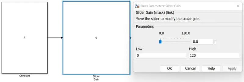
With slider gain, we can vary the speed while running the simulation and will get the results accordingly.

The model circuit of the drive cycle input with the above-mentioned blocks shown below

Distance Calculator Subsystem: -

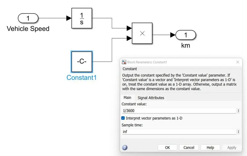
This subsystem is created to calculate the distance traveled by the vehicle during the simulation, here used an integrator block that gets the input signal of speed in km/hr from the vehicle body, and a constant block gave the value 1/3600 (hr to sec). Both the block combined by using the product block will result in the distance in km. The output of the product block is connected to the scope and display block to visualize the value.

Other Blocks Used for Modeling: -

1. Constant Block:

The Constant block generates a real or complex constant value signal. Use this block to provide a constant signal input. The block generates scalar, vector, or matrix output, depending on:

• The dimensionality of the Constant value parameter
• The setting of the Interpret vector parameters as 1-D parameter

The output of the block has the same dimensions and elements as the Constant value parameter. If you specify for this parameter a vector that you want the block to interpret as a vector, select the Interpret vector parameters as a 1-D check box. Otherwise, if you specify a vector for the Constant value parameter, the block treats that vector as a matrix.

2. Powergui:

The powergui block allows you to choose one of these methods to solve your circuit:

• Continuous, which uses a variable-step solver from Simulink.
• Discretization of the electrical system for a solution at fixed time steps.
• Phasor solution.

The powergui block also opens tools for steady-state and simulation results analysis and for advanced parameter design. You need the powergui block to simulate any Simulink model containing Simscape Electrical Specialized Power Systems blocks. It stores the equivalent Simulink circuit that represents the state-space equations of the model.

3.Simulink-PS Converter & PS Converter -Simulink:

• The Simulink-PS Converter block converts the input Simulink signal into a physical signal. Use this block to connect Simulink sources or other Simulink blocks to the inputs of a Physical Network diagram.
• The PS-Simulink Converter block converts a physical signal into a Simulink output signal. Use this block to connect outputs of a Physical Network diagram to Simulink scopes or other Simulink blocks.

4. Terminator:

Use the Terminator block to cap blocks whose output ports do not connect to other blocks. If you run a simulation with blocks having unconnected output ports, Simulink issues warning messages. Using Terminator blocks to cap those blocks helps prevent warning messages.

5. Scope:

The Simulink Scope block and DSP System Toolbox Time Scope block display time-domain signals.

6. Display:

The Display block shows the value of the input data. You can specify the frequency of the display. For numeric input data, you can also specify the format of display.

SIMULATION MODEL OF ELECTRIC CAR

Results:

1.FTP75

From the selector switch keep the constant value as ‘1’then the FTP75 driving cycle will be the drive input to the driver, run the simulation for T= 2474 secs and the simulation results shown below

The simulation result of Drive cycle vs Vehicle speed

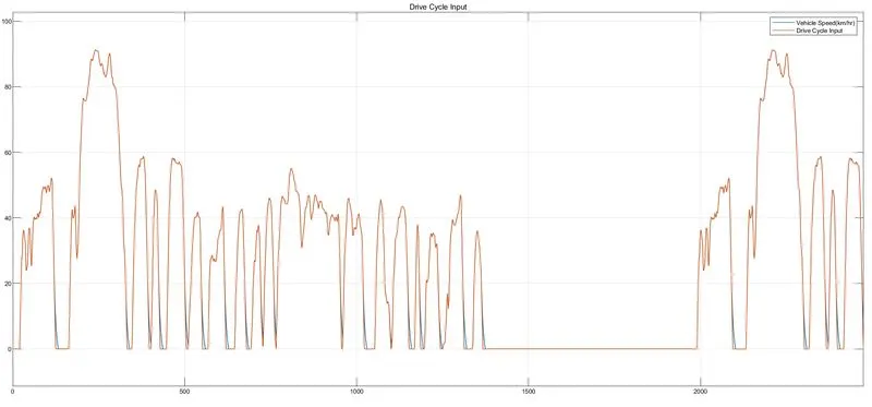
While the acceleration period, the designed vehicle achieved the max speed of the drive cycle.

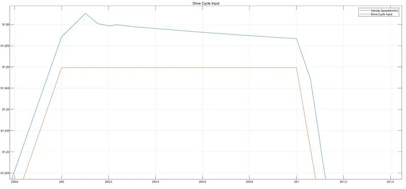
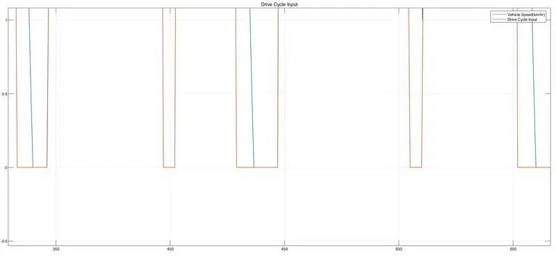
While deceleration or by applying the brakes there is a delay of 10sec to achieve the drive cycle it is due to the moment inertia of the vehicle as shown below

The battery SOC estimation for the entire simulation period is shown below, we can see that rise and downs of the battery SOC mean discharge and charging of the battery when the deceleration or by applying the brakes of the vehicle.

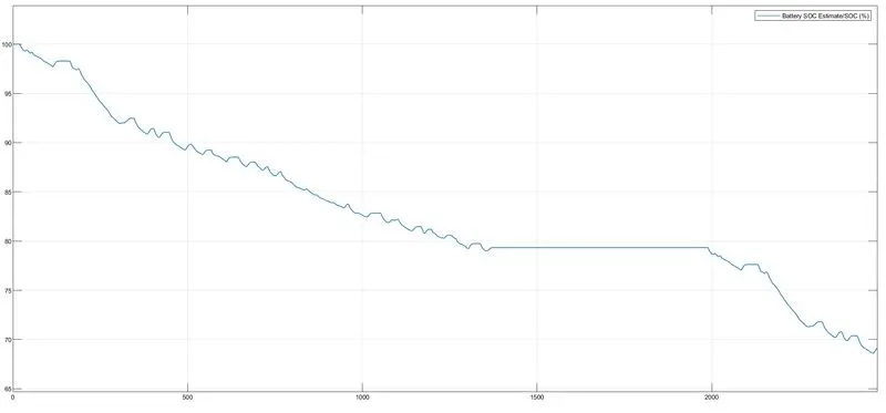
Throughout the simulation period, the SOC of the battery reduced from 100% to 69.2%

The discharging and charging of the current can be visualized from the Battery current plot, the +ve current value considered as discharging, and the -ve current value considered as the charging current of the battery which will be possible by the bi-directional converters.

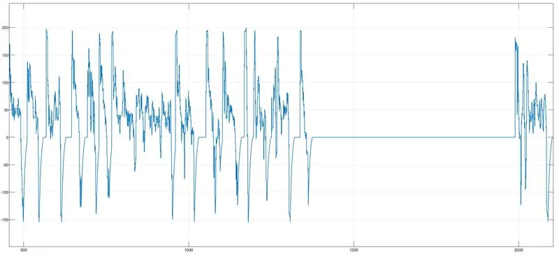
At the end of the simulation, the current value will be in -ve value to 0 which means the vehicle is in off condition and require to charge the battery.

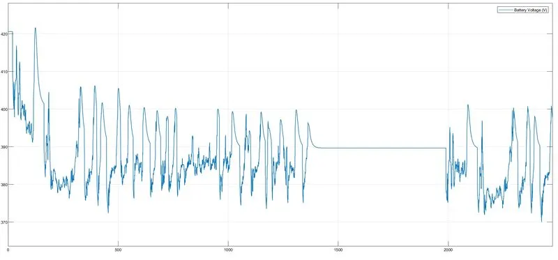
The battery voltage plot is shown below as the initial voltage will be more than the nominal voltage

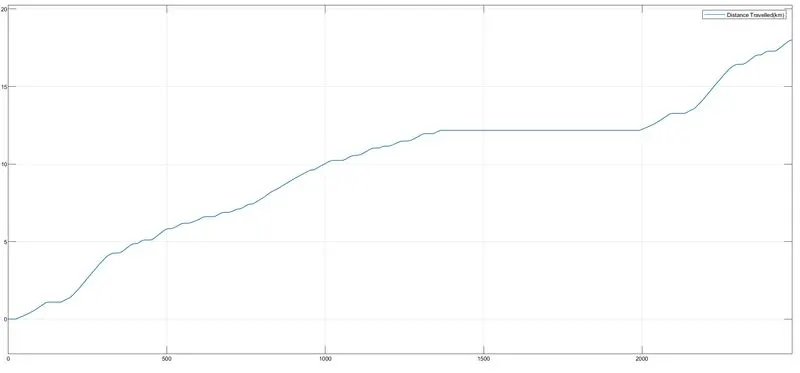
The distance traveled through the simulation period of T= 2474 secs is 18.01km

2. SIGNAL BUILDER

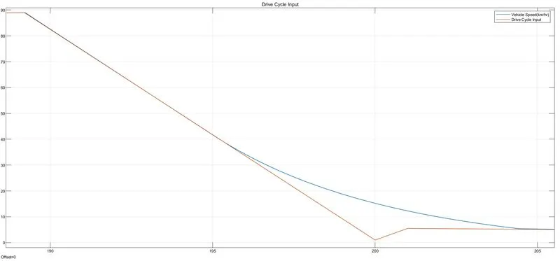
From the selector switch keep the constant value as ‘2’then the Signal Builder driving cycle will be the drive input to the driver, run the simulation for T= 600 secs and the simulation results shown below

The simulation result of Drive cycle vs Vehicle speed

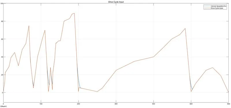
While the acceleration period, the designed vehicle achieved the max speed of the drive cycle.

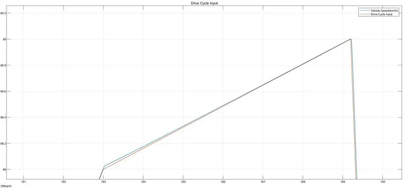
From the top speed of the vehicle then after applying the brakes to decelerate to 0 speed and again accelerate to move the vehicle, for a 20secs period in the deceleration period vehicle speed deviated from drive input and again continued with the drive cycle input as shown below

The battery SOC estimation for the entire simulation period is shown below, we can see that rise and downs of the battery SOC mean discharge and charging of the battery when the deceleration or by applying the brakes of the vehicle.

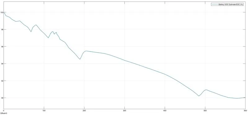
Throughout the simulation period, the SOC of the battery reduced from 100% to 90.04%

The discharging and charging of the current can be visualized from the Battery current plot and the battery voltage plot shown below

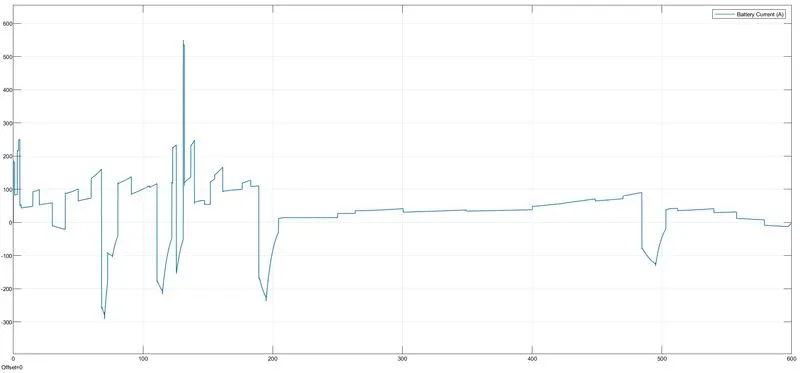
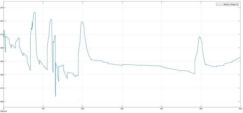
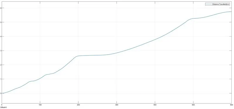
The distance traveled through the simulation period of T= 600 secs is 5.739km

3. From Spreadsheet

From the selector switch keep the constant value as ‘3’then the From Spreadsheet driving cycle will be the drive input to the driver, run the simulation for T= 600 secs and the simulation results shown below

The simulation result of Drive cycle vs Vehicle speed

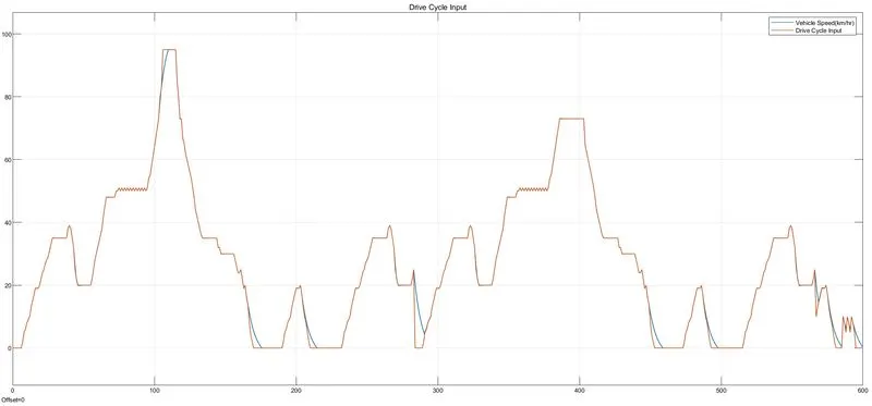
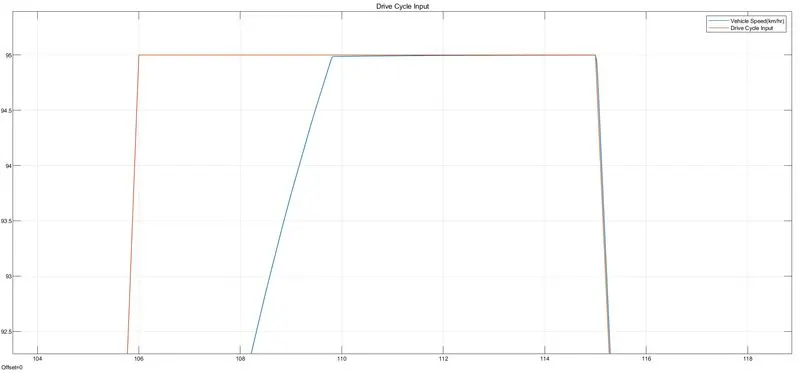
While at the top speed of the drive input, vehicle speed was achieved with the delay of 2 secs as shown below

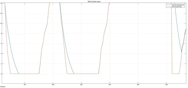
While deceleration from the top speed of the drive input, vehicle speed follows it the speed =15km/hr then after when the drive input reached 0 speed, the vehicle speed is achieved with the delay of 5 secs and if the drive input speed is for 0 speed for less than 5 secs and accelerate then vehicle speed continued to accelerate with the drive input without reaching 0 speed as shown in below plot.

The battery SOC estimation for the entire simulation period is shown below, we can see that rise and downs of the battery SOC mean discharge and charging of the battery when the deceleration or by applying the brakes of the vehicle.

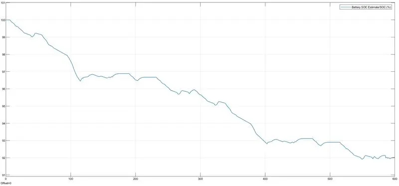
Throughout the simulation period, the SOC of the battery reduced from 100% to 90.04%

The discharging and charging of the current can be visualized from the Battery current plot and the battery voltage plot shown below

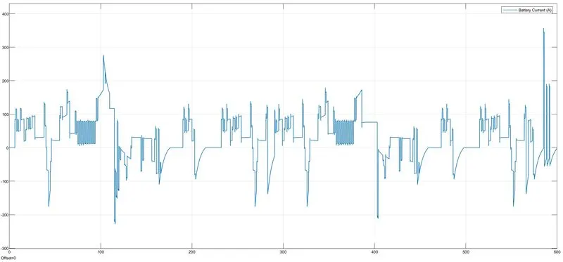
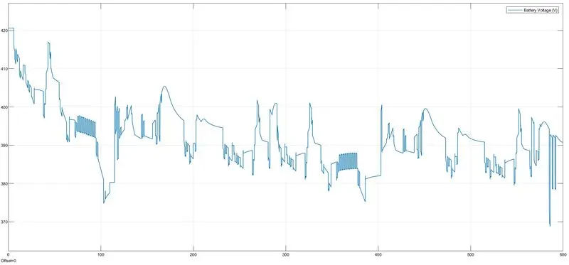
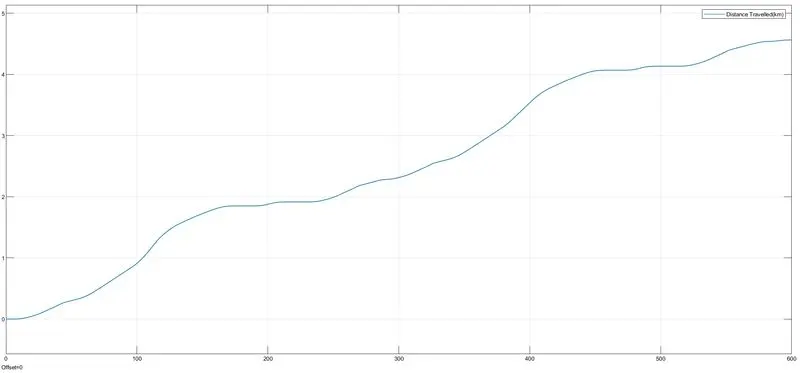
The distance traveled through the simulation period of T= 600 secs is 4.565km

4. Slider Gain

From the selector switch keep the constant value as ‘4’then the Slider gain driving cycle will be the drive input to the driver, given the slider gain max range as 120 km/hr, run the simulation for T= inf secs, varying the speed while simulation running and stopped the simulation at T=560 secs and the simulation results are shown below

The simulation result of Drive cycle vs Vehicle speed

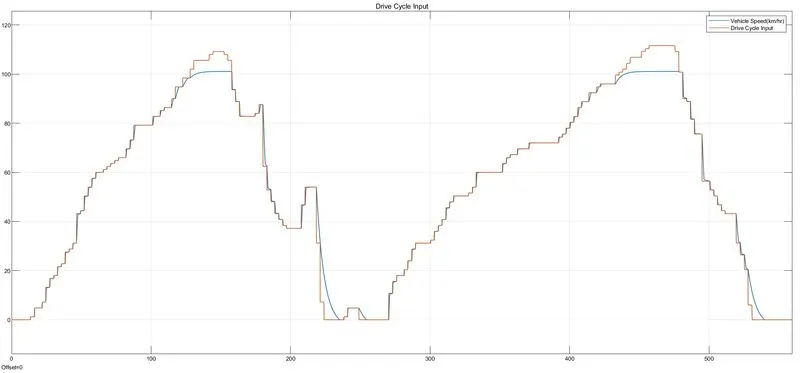
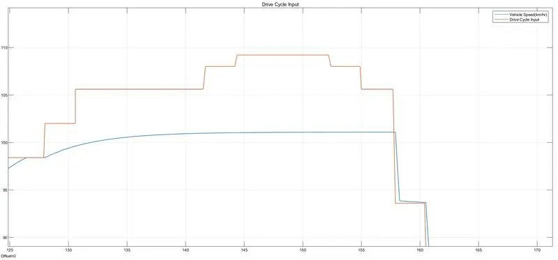
When the drive input tried to reach the top speed of 120km/hr, the vehicle speed reached a max speed of 101km/hr with the designed parameters of the EV car as shown below

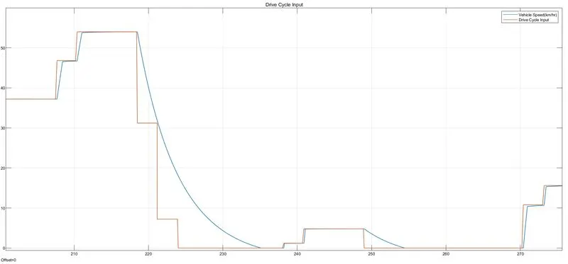
While deceleration or by applying the brakes of the vehicle, there is a delay of 15sec for the vehicle to achieve the drive cycle speed of 0km/hr it is due to the moment inertia of the vehicle as shown below

The battery SOC estimation for the entire simulation period is shown below, we can see that rise and downs of the battery SOC mean discharge and charging of the battery when the deceleration or by applying the brakes of the vehicle.

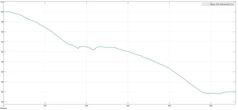
Throughout the simulation period, the SOC of the battery reduced from 100% to 83.97%

The discharging and charging of the current can be visualized from the Battery current plot and the battery voltage plot shown below

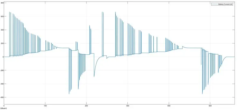
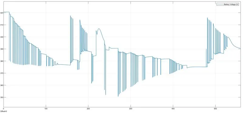
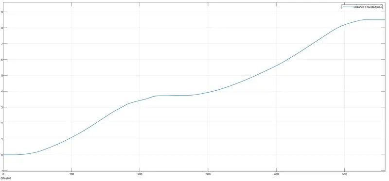
The distance traveled through the simulation period of T= 560 secs is 8.526km

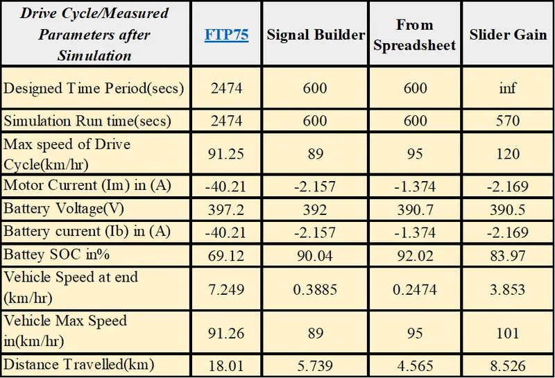
Consolidation of the Results

Advantages of Electric Car

The advantages of the Electric Car include:

Distance – The travel distance between every recharge is almost up to 150 – 180km before the battery gets drained.

Environment – No Greenhouse gases emitting such as CO2, NOx, and PM10s.

Fuel – No Oil Consumption by the vehicle.

Convenience – Recharge of the Cars as per the customer’s convenience will be provided soon. An electric grid will be available in close proximity either in the parking lot or the customer’s residence which will help in charging the car overnight while in parking.

Cost Effective – Due to the long-lasting battery technology, Electric Cars have more cost-effective batteries than regular cars.

Maintenance – Compared to regular cars, Electric Cars are cheaper to maintain.

Pollution – With a silent engine, there is less noise pollution.

Disadvantages of Electric Car

The disadvantages of Electric cars include:

Range – Not all Electric Vehicles have long distance range. On a full charge, most EVs run 60 to 100 miles, with very few small Electric Cars that can run anywhere between a 200 to 300 mile range.

Time Consuming – A full recharge usually takes an overnight time compared to the fuel filling which can happen in a few minutes. This becomes time-consuming when there are emergencies although there are tool kits that are available in the market for faster recharge and bringing down the time.

Initial Investment – It’s a huge investment for an initial purchase of the car along with the additional tool kits when compared to the Fuel Cars.

Inconsistency – Not all countries have adopted the Electric car in the market. Hence the charging stations are inconsistence. Although some countries have considerable market growth in this segment, the frequency of charging stations found is less. This makes it difficult for the consumers.

Restricted Choice – The choices of Electric Cars in the market have increased considerably when compared to the previous few decades. But as compared to the other models, the variety of cars has been restricted.

CONCLUSION:

In conclusion, the EV model has been created with the necessary block components using the SIMULINK software and the model has been simulated for a customized FTP75 drive cycle, Signal Builder, From Spreadsheet, and Slider gain. The simulation has produced results of the velocity of the vehicle, the current flowing from the battery, and the SOC of the battery as well as the distance traveled by the EV. Since the EV model was parameterized to simulate averaged voltage pulses in the H-Bridge and Controlled PWM voltage blocks to be fed into the DC motor, the simulation finished very quickly. While using the Slider gain kept the simulation pace for 10secs so that varying speed and generating simulation results. The EV model was able to follow the commands given by the reference velocities from the drive cycle data, although it could have followed the reference signals more closely.

Model file, screenshots of the model, results, and project word file consolidated zip file attached.