Final Project: Design of an Electric Vehicle

PROJECT : DESIGN OF ELECTRIC VEHICLE

EV HISTORY & THERORY:

Electric motive power started in 1827, when Hungarian priest Ányos Jedlik built the first crude but viable electric motor, provided with stator, rotor and commutator; the next year, he used it to power a tiny car. In 1835, professor Sibrandus Stratingh of the University of Groningen, the Netherlands, built a small-scale electric car, and between 1832 and 1839 (the exact year is uncertain), Robert Anderson of Scotland invented the first crude electric carriage, powered by non-rechargeable primary cells. American blacksmith and inventor Thomas Davenport built a toy electric locomotive, powered by a primitive electric motor, in 1835. In 1838, a Scotsman named Robert Davidson built an electric locomotive that attained a speed of four miles per hour (6 km/h). In England a patent was granted in 1840 for the use of rails as conductors of electric current, and similar American patents were issued to Lilley and Colten in 1847.The first mass-produced electric vehicles appeared in America in the early 1900s. In 1902, the Studebaker Automobile Company entered the automotive business with electric vehicles, though it also entered the gasoline vehicles market in 1904. However, with the advent of cheap assembly line cars by Ford Motor Company, the popularity of electric cars declined significantly.

Due to lack of electricity grids and the limitations of storage batteries at that time, electric cars did not gain much popularity; however, electric trains gained immense popularity due to their economies and achievable speeds. By the 20th century, electric rail transport became commonplace due to advances in the development of electric locomotives. Over time their general-purpose commercial use reduced to specialist roles as platform trucks, forklift trucks, ambulances, tow tractors and urban delivery vehicles, such as the iconic British milk float; for most of the 20th century, the UK was the world's largest user of electric road vehicles.Electrified trains were used for coal transport, as the motors did not use precious oxygen in the mines. Switzerland's lack of natural fossil resources forced the rapid electrification of their rail network. One of the earliest rechargeable batteries – the nickel-iron battery – was favored by Edison for use in electric cars.

EVs were among the earliest automobiles, and before the pre-eminence of light, powerful internal combustion engines, electric automobiles held many vehicle land speed and distance records in the early 1900s. They were produced by Baker Electric, Columbia Electric, Detroit Electric, and others, and at one point in history out-sold gasoline-powered vehicles. In 1900, 28 percent of the cars on the road in the US were electric. EVs were so popular that even President Woodrow Wilson and his secret service agents toured Washington, D.C. in their Milburn Electrics, which covered 60–70 mi (100–110 km) per charge.Most producers of passenger cars opted for gasoline cars in the first decade of the 20th century, but electric trucks were an established niche well into the 1920s.A number of developments contributed to a decline in the popularity of electric cars. Improved road infrastructure required a greater range than that offered by electric cars, and the discovery of large reserves of petroleum in Texas, Oklahoma, and California led to the wide availability of affordable gasoline/petrol, making internal combustion powered cars cheaper to operate over long distances. Electric vehicles were not seldom marketed as a women’s luxury car, which may have been a stigma among male consumers. Also, internal combustion powered cars became ever-easier to operate thanks to the invention of the electric starter by Charles Kettering in 1912, which eliminated the need of a hand crank for starting a gasoline engine, and the noise emitted by ICE cars became more bearable thanks to the use of the muffler, which Hiram Percy Maxim had invented in 1897. As roads were improved outside urban areas, electric vehicle range could not compete with the ICE. Finally, the initiation of mass production of gasoline-powered vehicles by Henry Ford in 1913 reduced significantly the cost of gasoline cars as compared to electric cars.In the 1930s, National City Lines, which was a partnership of General Motors, Firestone, and Standard Oil of California purchased many electric tram networks across the country to dismantle them and replace them with GM buses. The partnership was convicted of conspiring to monopolize the sale of equipment and supplies to their subsidiary companies, but were acquitted of conspiring to monopolize the provision of transportation services.

During the late 20th and early 21st century, the environmental impact of the petroleum-based transportation infrastructure, along with the fear of peak oil, led to renewed interest in an electric transportation infrastructure’s differ from fossil fuel-powered vehicles in that the electricity they consume can be generated from a wide range of sources, including fossil fuels, nuclear power, and renewables such solar power and wind power or any combination of those. The carbon footprint and other emissions of electric vehicles varies depending on the fuel and technology used for electricity generation.The electricity may be stored in the vehicle using a battery, flywheel, or supercapacitors. Vehicles using internal combustion engines usually only derive their energy from a single or a few sources, usually non-renewable fossil fuels. A key advantage of electric vehicles is regenerative braking, which recovers kinetic energy, typically lost during friction braking as heat, as electricity restored to the on-board battery.

COMPONENTS:

Major component used are as below:

• Wheel/tier
• Vehicle body
• Battery system
• Transmission Sytem
• Power Converter
• Motor Controller

Main Simulation:

The below image shows the simulink design of complete EV. By using the above mention block the design is made.The Drive cycle block is used to give input to the vehicle & accleration / deceration inputs are given.

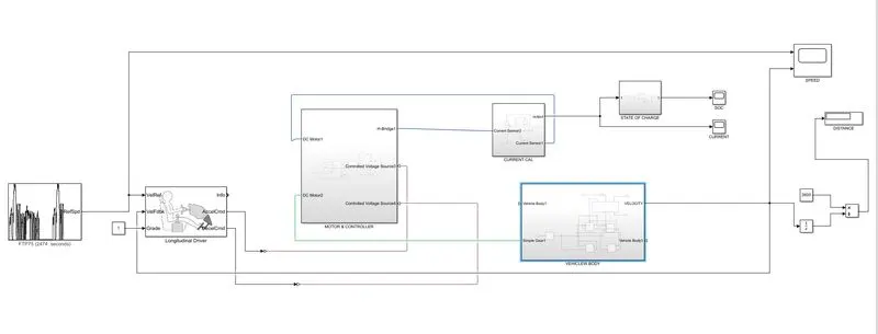
Now let us look in details each block used in Simulation and their paramaters:

VEHICLE BODY:

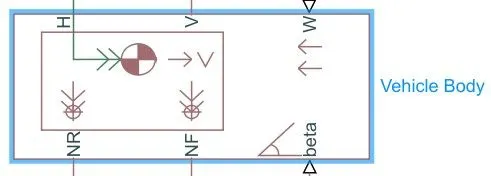
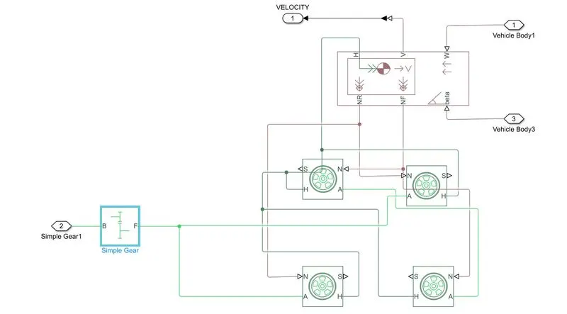
Represents a two-axle vehicle body in longitudinal motion. The block accounts for body mass, aerodynamic drag, road incline, and weight distribution between axles due to acceleration and road profile. The vehicle can have the same or a different number of wheels on each axle. Optionally include pitch and suspension dynamics or additional variable mass and inertia. The vehicle does not move vertically relative to the ground.

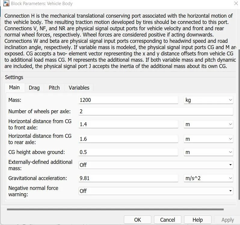
Connection H is the mechanical translational conserving port associated with the horizontal motion of the vehicle body. The resulting traction motion developed by tires should be connected to this port. Connections V, NF, and NR are physical signal output ports for vehicle velocity and front and rear normal wheel forces, respectively. Wheel forces are considered positive if acting downwards. Connections W and beta are physical signal input ports corresponding to headwind speed and road inclination angle, respectively. If variable mass is modeled, the physical signal input ports CG and M are exposed. CG accepts a two- element vector representing the x and y distance offsets from vehicle CG to additional load mass CG. M represents the additional mass. If both variable mass and pitch dynamics are included, the physical signal port J accepts the inertia of the additional mass about its own CG.

The parameters selected are as below:

TIRE:

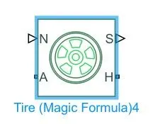
Represents the longitudinal behavior of a highway tire characterized by the tire Magic Formula. The block is built from Tire-Road Interaction (Magic Formula) and Simscape Foundation Library Wheel and Axle blocks. Optionally, the effects of tire inertia, stiffness, and damping can be included.

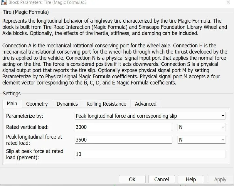
Connection A is the mechanical rotational conserving port for the wheel axle. Connection H is the mechanical translational conserving port for the wheel hub through which the thrust developed by the tire is applied to the vehicle. Connection N is a physical signal input port that applies the normal force acting on the tire. The force is considered positive if it acts downwards. Connection S is a physical signal output port that reports the tire slip. Optionally expose physical signal port M by setting Parameterize by to Physical signal Magic Formula coefficients. Physical signal port M accepts a four element vector corresponding to the B, C, D, and E Magic Formula coefficients.

The parameters selected are as below:

SIMPLE GEAR:

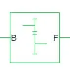
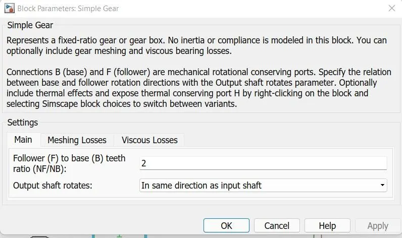
Represents a fixed-ratio gear or gear box. No inertia or compliance is modeled in this block. You can optionally include gear meshing and viscous bearing losses.

Connections B (base) and F (follower) are mechanical rotational conserving ports. Specify the relation between base and follower rotation directions with the Output shaft rotates parameter. Optionally include thermal effects and expose thermal conserving port H by right-clicking on the block and selecting Simscape block choices to switch between variants.

VEHICLE BODY SUBSYSTEM:

By using all above blocks a susbsytem is created. All the component are connected to their respective terminal and whole system is created as a subsytem of EV which is as below.

STATE OF CHARGE:

The below system shows the calcultion of SOC:

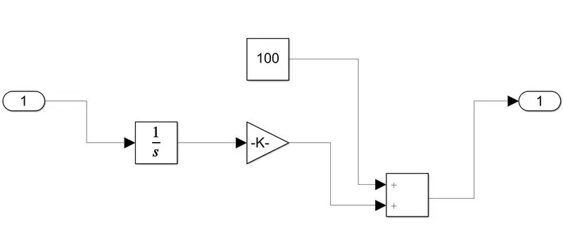
The blocks used are:

• Integrator:Continuous-time integration of the input signal.
• Gain:Element-wise gain (y = K.*u) or matrix gain (y = K*u or y = u*K).
• Add:

  Add or subtract inputs. Specify one of the following:

  a) character vector containing + or - for each input port, | for spacer between ports (e.g. ++|-|++)

  b) scalar, >= 1, specifies the number of input ports to be summed.

  When there is only one input port, add or subtract elements over all dimensions or one specified dimension

• Constant: To take refrence as battery 100% charge

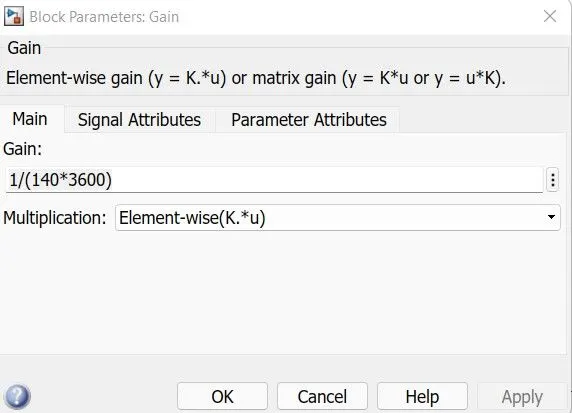
140Ah And 3600 sec.

Futher this block output is connected to the scope and the SOC is observed.

MOTOR CONTROLLER SUBSYSTEM:

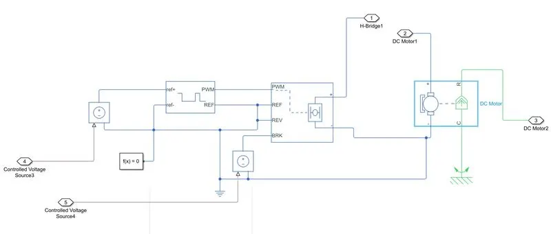
The major blocks used in the subsystem are as below:

• DC motor
• Controlled PWM Voltage.
• H-Bridge

Now let us look at each block in details:

DC MOTOR:

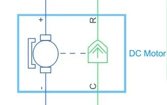
This block represents the electrical and torque characteristics of a DC motor.

The block assumes that no electromagnetic energy is lost, and hence the back-emf and torque constants have the same numerical value when in SI units. Motor parameters can either be specified directly, or derived from no-load speed and stall torque. If no information is available on armature inductance, this parameter can be set to some small non-zero value.

When a positive current flows from the electrical + to - ports, a positive torque acts from the mechanical C to R ports. Motor torque direction can be changed by altering the sign of the back-emf or torque constants.

The parameters are kept as below:

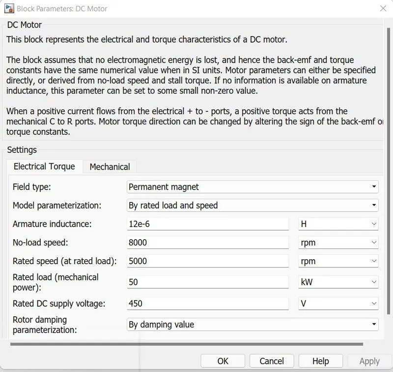
The motors used in EV are huge hence 50KW is selected with Rated speed of 5000 rpm.

The DC motor is connected to Mechanical Ref:

This block represents a mechanical rotational reference point, that is, a frame or a ground. Use it to connect mechanical rotational ports that are rigidly affixed to the frame (ground).

H-BRIDGE:

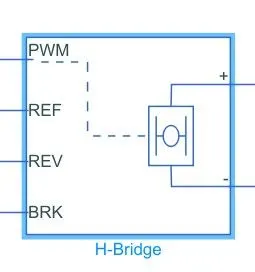
This block represents an H-bridge motor drive. The block can be driven by the Controlled PWM Voltage block in PWM or Averaged mode. In PWM mode, the motor is powered if the PWM port voltage is above the Enable threshold voltage. In Averaged mode, the PWM port voltage divided by the PWM signal amplitude parameter defines the ratio of the on-time to the PWM period. Using this ratio and assumptions about the load, the block applies an average voltage to the load that achieves the correct average load current. The Simulation mode parameter value must be the same for the Controlled PWM Voltage and H-Bridge blocks.

If the REV port voltage is greater than the Reverse threshold voltage, then the output voltage polarity is reversed. If the BRK port voltage is greater than the Braking threshold voltage, then the output terminals are short circuited via one bridge arm in series with the parallel combination of a second bridge arm and a freewheeling diode. Voltages at ports PWM, REV and BRK are defined relative to the REF port.

If exposing the power supply connections, the block only supports PWM mode.

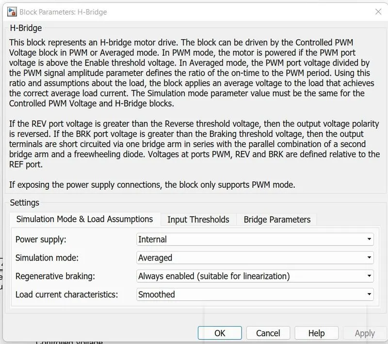
The Simulation mode is kept averaged for faster simulation & the regenerative braking is enabled.

CONTROLLED PWM VOLTAGE:

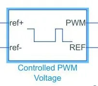
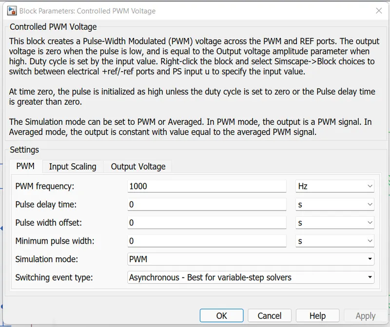
This block creates a Pulse-Width Modulated (PWM) voltage across the PWM and REF ports. The output voltage is zero when the pulse is low, and is equal to the Output voltage amplitude parameter when high. Duty cycle is set by the input value. Right-click the block and select Simscape->Block choices to switch between electrical +ref/-ref ports and PS input u to specify the input value.At time zero, the pulse is initialized as high unless the duty cycle is set to zero or the Pulse delay time is greater than zero.The Simulation mode can be set to PWM or Averaged. In PWM mode, the output is a PWM signal. In Averaged mode, the output is constant with value equal to the averaged PWM signal.

CONTROLLED VOLTAGE SOURCE:

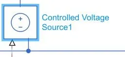
The block represents an ideal voltage source that is powerful enough to maintain the specified voltage at its output regardless of the current passing through it. The output voltage is V = Vs, where Vs is the numerical value presented at the physical signal.

CURRENT CALCULATION:

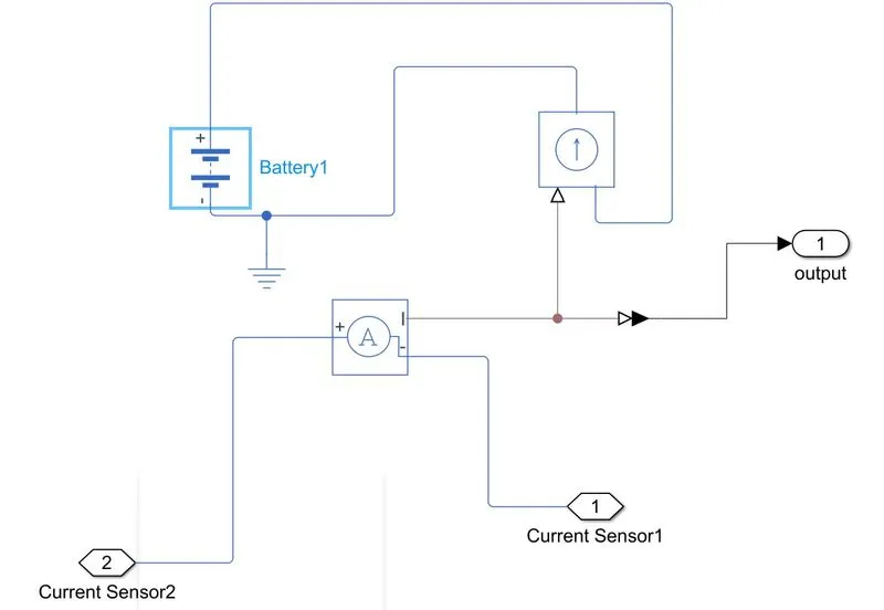
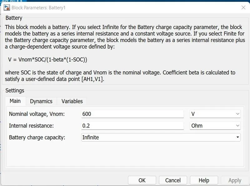
BATTERY :

This block models a battery. If you select Infinite for the Battery charge capacity parameter, the block models the battery as a series internal resistance and a constant voltage source. If you select Finite for the Battery charge capacity parameter, the block models the battery as a series internal resistance plus a charge-dependent voltage source defined by:

V = Vnom*SOC/(1-beta*(1-SOC))

where SOC is the state of charge and Vnom is the nominal voltage. Coefficient beta is calculated to satisfy a user-defined data point [AH1,V1].

CURRENT SENSOR:

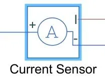
The block represents an ideal current sensor, that is, a device that converts current measured in any electrical branch into a physical signal proportional to the current.

Connections + and - are conserving electrical ports through which the sensor is inserted into the circuit. Connection I is a physical signal port that outputs current value.

LONGITUDINAL DRIVER:

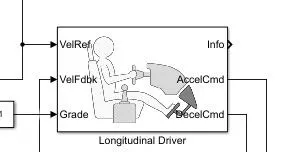
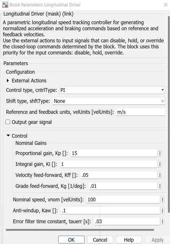
A parametric longitudinal speed tracking controller for generating normalized acceleration and braking commands based on reference and feedback velocities.

Use the external actions to input signals that can disable, hold, or override the closed-loop commands determined by the block. The block uses this priority for the input commands: disable, hold, override.

DRIVE CYCLE BLOCK:

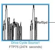
Generates a standard or user-specified longitudinal drive cycle. The block output is the vehicle longitudinal speed. You can import drive cycles from:

- Predefined sources

- Workspace variables, including arrays and time series objects

- mat, xls, xlsx, or txt files

Use the fault tracking parameters to identify drive cycle faults within specified speed and time tolerances.

RESULTS:

The above whole model is simulated by using the FTP75 cycle. According to that the simulation time is set.The Output obtain are in scope which are SOC,Current,Speeed and Distance in Display.

SPEED SCOPE:

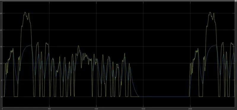
Their are two signal.Theblue signal is the vehicle body speed and the yellow signal is the FTP drive cycle data.As we see the longitudinal driver maintain the drive cycle data,the controler cis working fine to maintain the acceleration and decceration effectively.

CURRENT SCOPE:

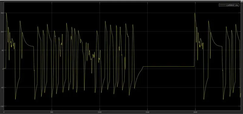
The current varies as per the acceleration and deceleration done by the driver.

SOC SCOPE:

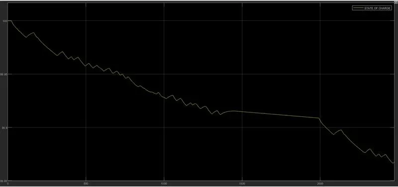
This scope shows how the battery is consumed during all the drive cycle. as well during regenerative braking small up peaks are seen.The SOC is at t=0 is 100% and at t=2474 is

DISTANCE:

The total distance travel by the EV by following the above drive cycle is 20 km

CONCLUSION:

The EV model is created by using the simulink blocks and powertrain.The model is simulated using FTP75 drive cycle with simukation time of 2474 sec.The simulations shows the output of SOC which observed during the simulation is 100% and at end 90% of the cycle. By completing the cycle EV travelled 20 km.The model was enabled with the regenrative braking which helps the battery to charge during braking.