Final Project: Design of an Electric Vehicle

Create a MATLAB model of an electric car that uses a battery and a DC motor. Choose suitable blocks from the Powertrain block set. Prepare a report about your model including the following:

Objectives:

1. System-level configurations

2. Model parameters

3. Results

4. Conclusion

#ANSWER :

A Battery operated vehicle is with no other source is called Electric Vehicle. the vehicles which uses other sources like fuel are known as hybrid electric vehicles( which have both IC engine and battery).

An electric vehicle exclusively uses the chemical energy which is stored in the battery Nowadays the fuels are limited and the petrol deisel are may not be available in future . these circumstances leads the interest towards the battery operated vehicles.

which are harmless for the nature and environment.

the cost per kilometer also reduces when compared with the gasoline vehicles.

Now in this Project, I have developed the simulink model which satisfies the all the conditions of electric vehicle system.

Here I developed a model which is simple and low run time model.

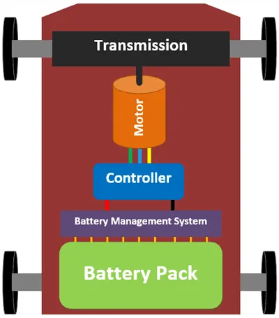
The basic components for modelling the electric vehicle in simulink are

1. Vehicle Body

2. Gear system

3. DC Motor

4. controller

5. power converter

6. Longitudinal Driver

7.Driving Cycle

8.Battery Pack

1. Vehicle Body:

The vehicle body contains wheels and physical design of the vehicle and the parameters of dimensions of the whole electric vehicle body and the gear system is included in the vehicle body block.

we are considering the tire (magic formula) which tells about the longitudinal behavior of the tire in highway .

which is built from the tire road interaction. we can include the effects of inertia and stiffness and damping also.

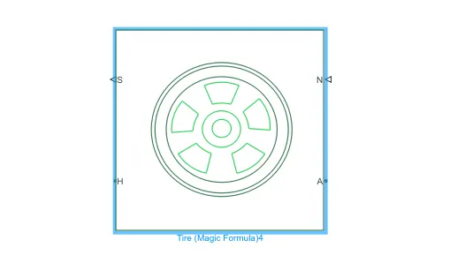
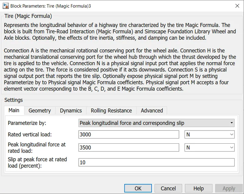
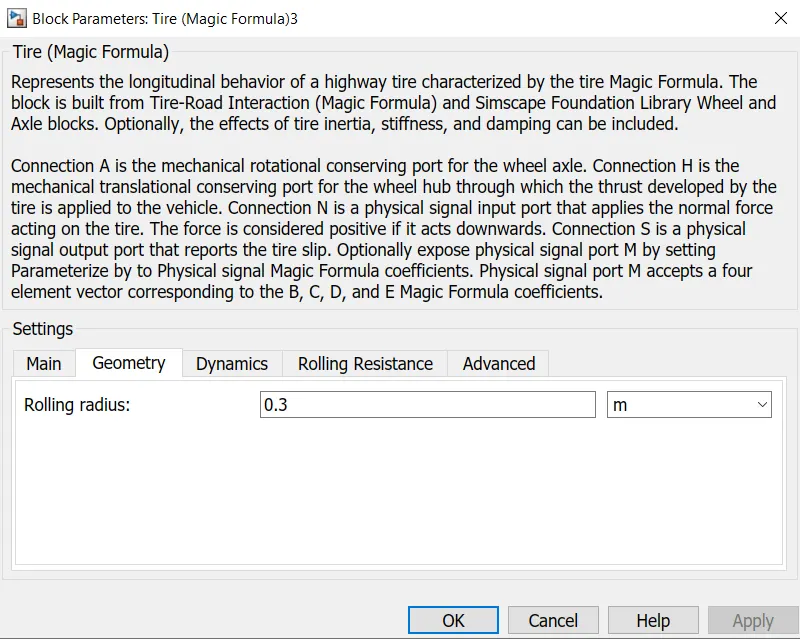
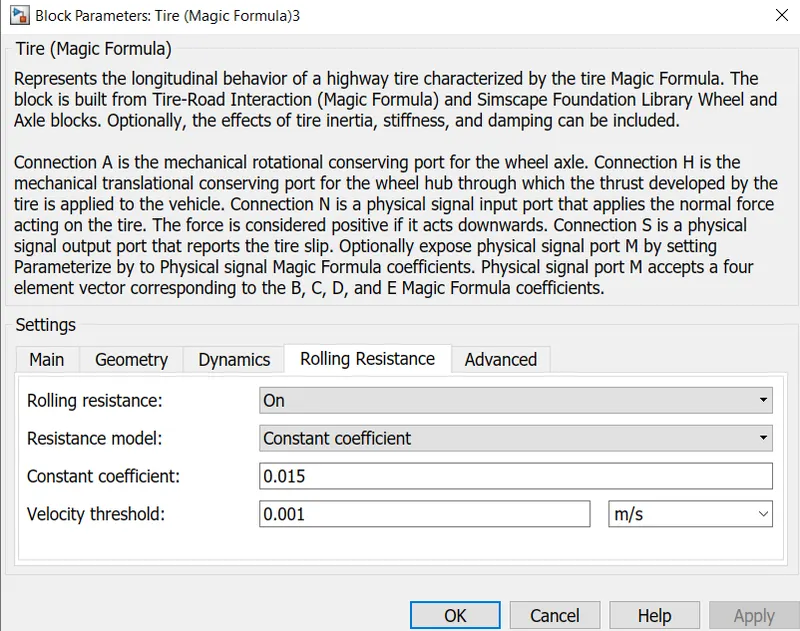
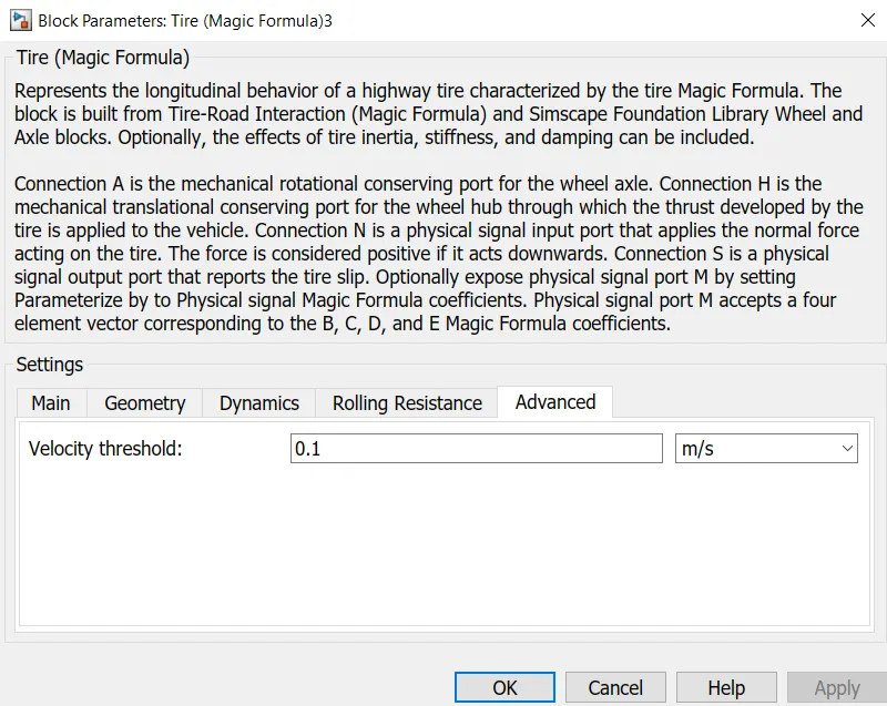
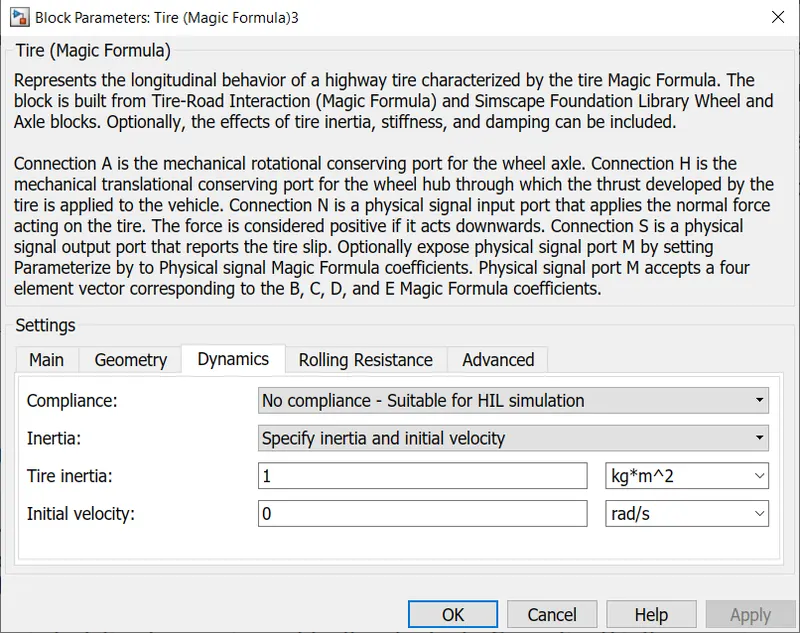
Connection A is the mechanical rotational conserving port Connection H is the mechanical translational conserving port for the wheel hub. Connection N is a physical signal input port that applies the normal force. Physical signal port M accepts a four-element vector corresponding to the B, C, D, and E Magic Formula coefficients. The force is considered positive if it acts downwards. Connection S is a physical signal output port that reports the tire slip.

Now we attach all hubs to vehicle body , the simulink block of vehicle body is

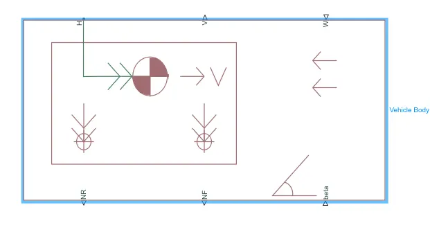
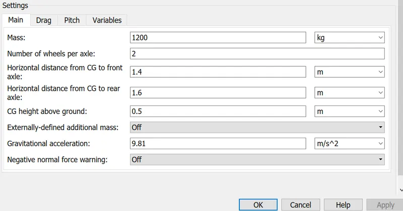
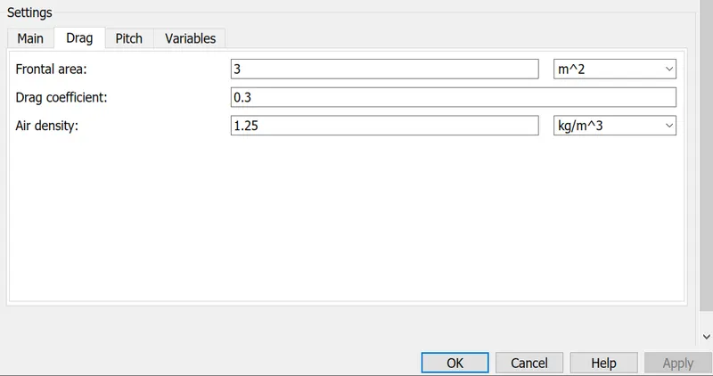
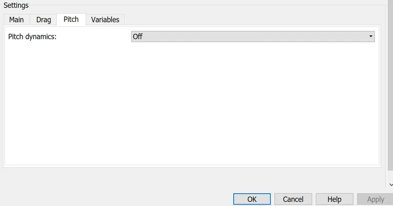
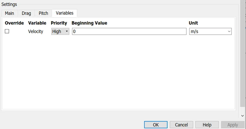
above image shows a two-axle vehicle in longitudinal motion. It consists body mass, road incline,aerodynamic drag, and weight distribution between axles due to acceleration and nature of road profile. Any number of wheels can be installed on the axle. it also consists pitch and suspension dynamics or additional variable inertia &mass. The vehicle does not move vertically relative to the ground.

Connection H is the mechanical translational conserving port . Connections V, NF, and NR are physical signal output ports for vehicle velocity and front and rear normal wheel forces, respectively. The forces of wheels are considered positive if acti downward direction. Connections W and beta are physical signal input ports corresponding to headwind speed and road inclination angle, respectively. If the variable mass is modeled, the physical signal input ports CG and M are exposed. CG accepts a two-element vector representing the x and y distance offsets from vehicle CG to additional load mass CG. M represents the additional mass. If both variable mass and pitch dynamics are included, the physical signal port J accepts the inertia of the additional mass about its own CG.

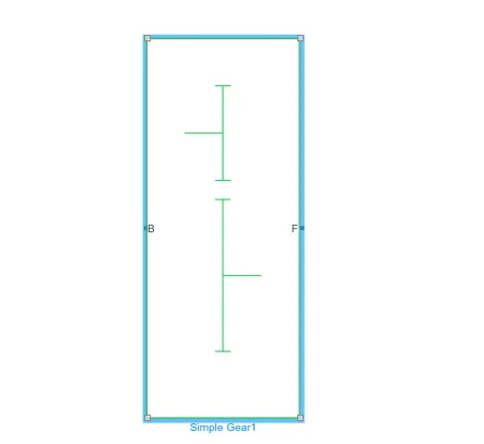
2.Simple Gear:

simple gear is the gear ratio. which does not account for inertia or compliance. viscous bearings and back lash

gearing mesh are included in this model.

3. DC Motor:

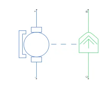
we can have the inbuilt model of Dc Motor, which is shown above.

* its duty is to convert the electrical energy into rotational mechanical energy

* we supply the power to the motor by Battery and using some other power converters.

*according to the given supply to the motor terminals , we can control the motor characteristics like speed .

*Here the motor field is created by permanent magnets . needs no electrical supply to energize the field of this motor.

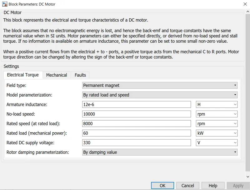
*The armature inductance and the mechanical parameters are given below values.

H-Bridge:

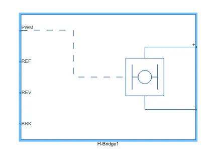
An H-bridge is an electronic circuit that switches the polarity of a voltage applied to a load. such circuits are used in robotics and other applications to allow DC motors to run backward & forward. we can control in all quadrants.

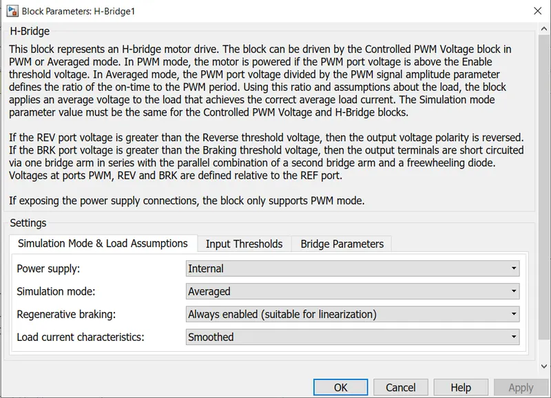
Here the power supply is internal. and we choose simulation mode averaged. this has to match the dc supply voltage of the

motor.

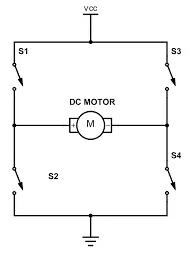from the above figure the four switches are controllable. and with their controllability we can supply the current in backward and forward direction. and so motor speed can be made positive and negative . which used for motoring and breaking applications.

Controlled PWM:

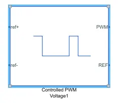
The Pwm and ref ports are corresponding connections to the H bridge circuit.

*The two references input nodes which corresponds to the inputs given from the longitudinal driver block.

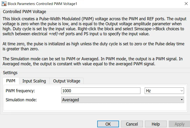
*The block generates the required voltage by manipulating the width of the pulse and as per the commands by pwm acceleration or decelaration takes place.

* here we are giving 1000hz frequency to the PWM block.

Longitudinal Driver:

Longitudinal drive block is inbuily in the simulink. from the powertrain block set.

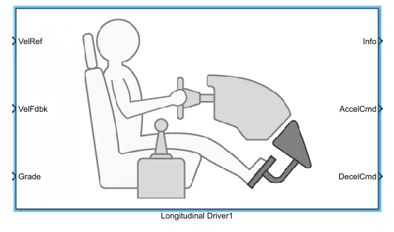
here vel Ref node represents the desired velocity to be driven ,

and VelFdbk node gives the actual velocity of the vehicle.

Grade represents is there any slope , we can include the gradeability also. but we are not considering in this simulation.

and according to the reference velocity and actual velocity , drive has to pass the commands of acceleration and decelaration to the PWM block.

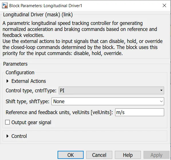
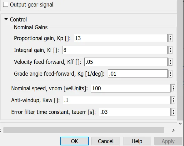
here we used PI controller, and the integral gain we are giving 8 and proportional gain as 13.

Driving Cycle:

driving cycle represents the plot between speed and time , we are now having so many data sets of driving cycle data in mathworks. like urban driving cycle in metro cities like that , in different regions with different traffic conditions there are lot of driving cycle data are available.

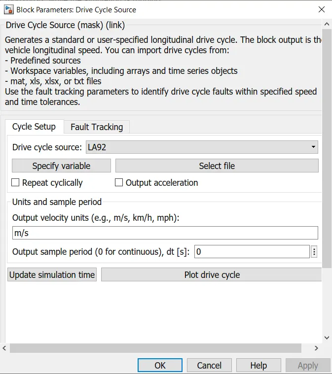
here we are considering the LA92 driving cycle ,

the plot of LA92 driving cycle is

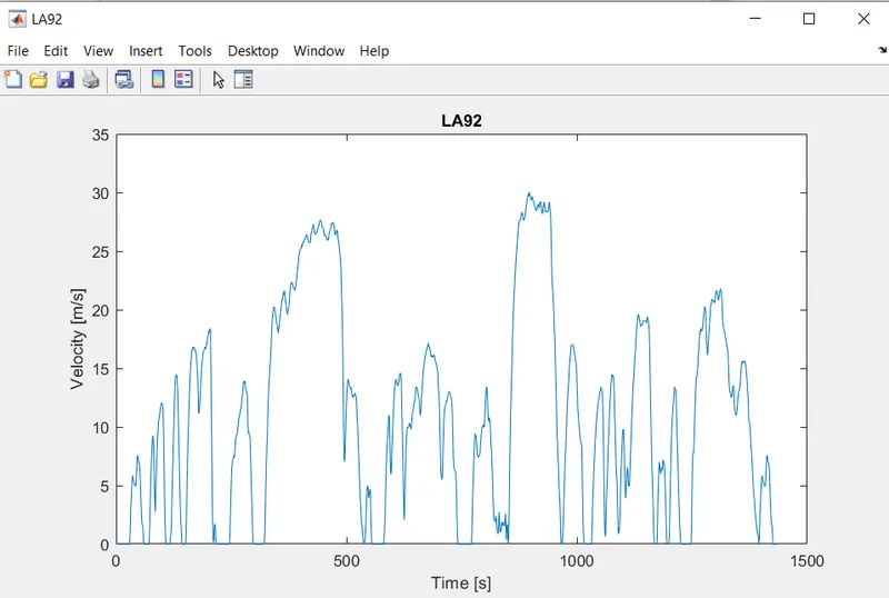
In the above plot we can observe acceleration and braking points . these references will be given to the longitudinal driver block.

Battery source:

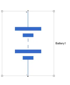
to reduce the simulation time we are considering the nominal battery voltage instead of SOC Block.

here we are giving 400V of supply and internal resistance of 1ohm.

providing amp hour rating of 50.

the resistance is connected in series to the battery .

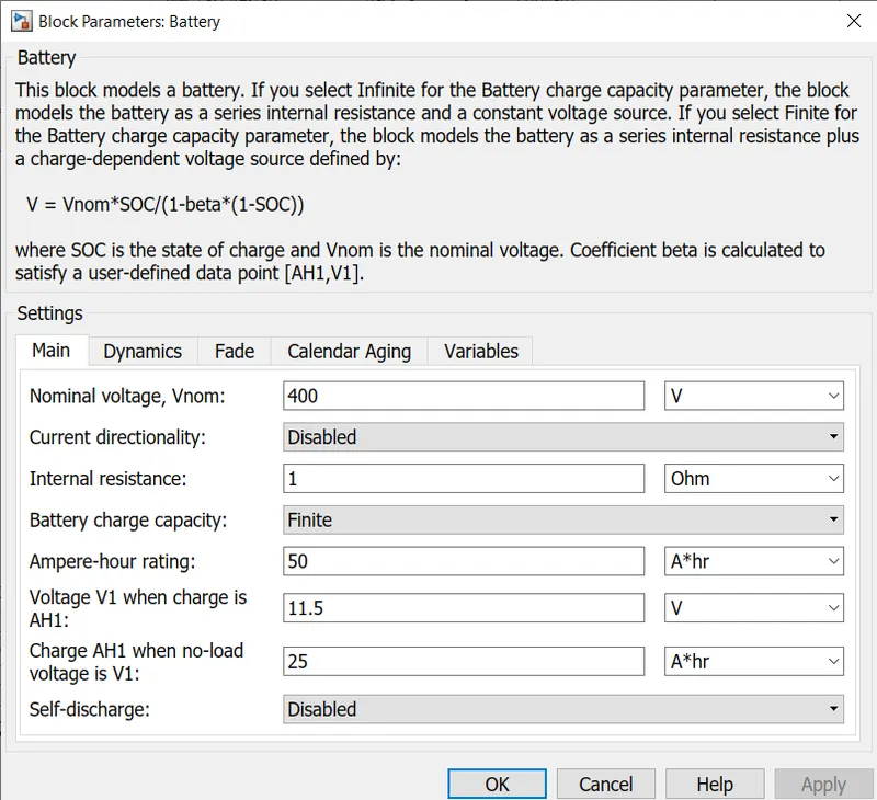
V = Vnom*SOC/(1-beta*(1-SOC))

where SOC is the state of charge and Vnom is the nominal voltage of the battery. beta is calculated to satisfy a user-defined data point [AH1,V1].

State of charge:

It tells about the how much percentage of charge remained in the battery pack.

we can estimate it by finding the stored charge in the battery.

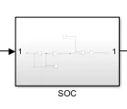
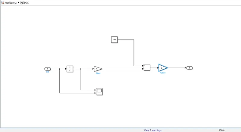
the current in the battery circuit is controlled by the current which goes inside of the dc motor and by knowing the current direction also the charge stored also changes .

the charge in the battery increases when the braking is applied and decreases when motoring operation occurs.

we know that integral of current flowing through a conductor gives the charge stored .

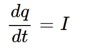
upon integrating the current we can find charge in the battery.

we need to convert the coloumbs of charge into Ah .

1 coloumb = 0.000278Ah.

we assumed 50 Ah rating . so we have to subtract the charge stored

and calculate the charge remained in percentage of 50Ah.

for example

at starting no energy is consumed from battery.

so (50Ah-0)/50Ah which is again multiplied with 100 to get remaining percentage of charge stored.

and the covered distance is measured by integrating the velocity.

which upon divided by 3600 to get the distance inKm.

The simulink model

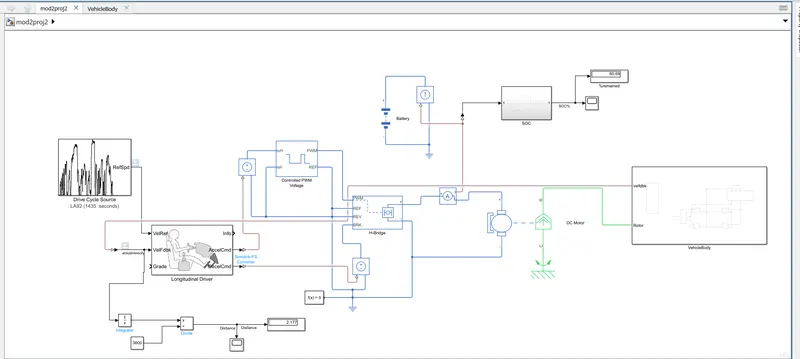
from the above image the blocks are connected as mentioned .

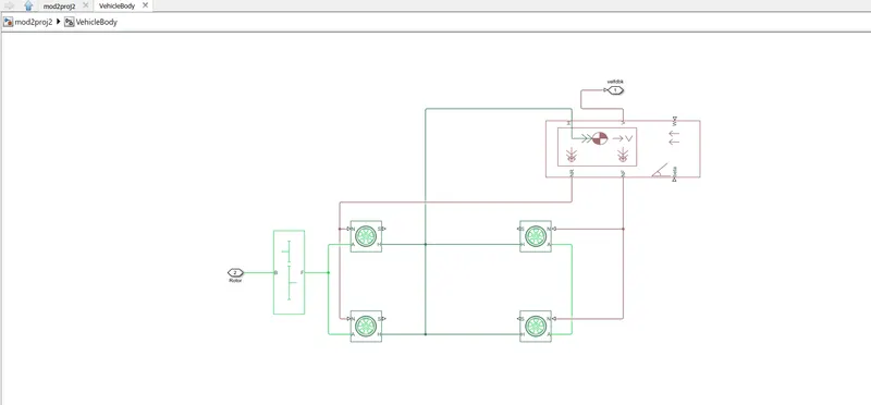
The above image is the subsystem of vehicle body.

which consistes all the tires and vehicle dimensions and connections with the gear box.

the results after simulation are given below.

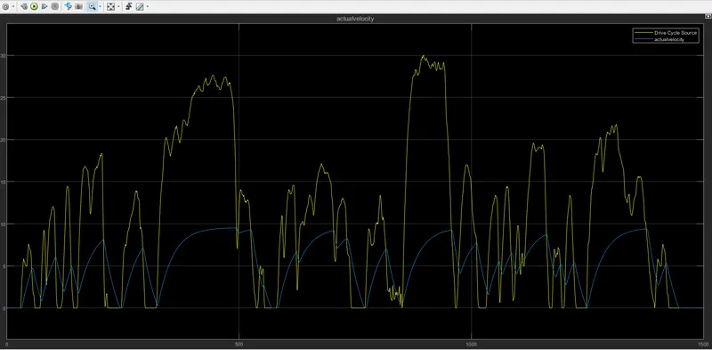
Observations:

* here we consider LA92 driving cycle, which is 1435 seconds long

* the driver gives the acceleration to the vehicle by comparing the reference speeds

* the reference speed from the driving cycle is more than the actual then the acceleration happens and viceversa

* we can observe this from the above graph.

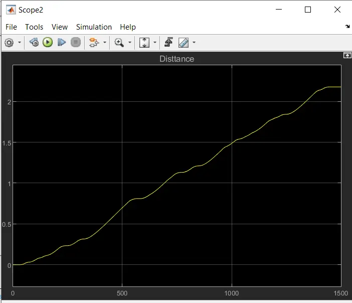
here we are having the distance curve which shows how many kilometers the vehicle covered with respect totime.

the total covered distance is 2.177kms.

..

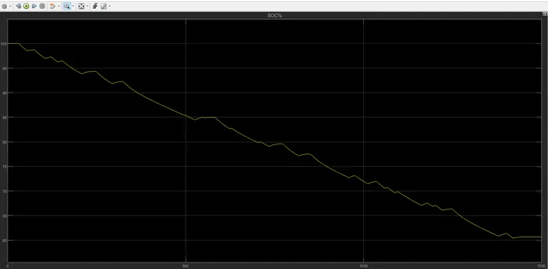
* The above curve gives the charging and discharging plot of the battery .

* we can observe at acceleration the soc discharges and at decelaration the soc charges back to the battery.

* The remaining SOC percentage of the battery is 60.69%.